Vocabulary, frequency and the OOV problem

The previous lesson, on tokenisation, left $V$ a finite list, and a finite list has a hole in it: sooner or later a token arrives that the list does not hold. That lesson named the hole; this one measures it. And measuring it means counting: not only which tokens a corpus contains, but how unevenly it uses them, because that is what decides how many arrivals fall through the hole.

That frequency distribution decides which tokens are worth keeping, which are reasonable to leave out, and so how often the model will meet a word outside its vocabulary, one that is out-of-vocabulary (OOV). The distribution has a strikingly unequal shape, and it is the same shape in every corpus and every language. That shape, not the size of the corpus and not the language, is what fixes how much text you can cover with a vocabulary that fits in memory.

Count the tokens of any English text and the same scene appears every time. At the head, a handful of pieces that never stop coming: the, and, to, in, and the punctuation. In the tail, a crowd that appears once in the whole text and never returns: librarian, cryptocurrency, monastery. In the toy corpus you will work with in this lesson (228 tokens in all), the most frequent appears 30 times, and 72 of the 107 distinct strings appear exactly once.

It is a single observation, and it pulls in two opposite directions. The frequent strings are so few that keeping all of them costs almost nothing; the rare ones are so many that keeping all of them is impossible. And the uncomfortable part is that almost everything you care about in a sentence lives in the tail: the proper nouns, the technical terms, the words coined last month.

The shape of a corpus's frequencies

Counting forces apart two things that have gone together until now. Apply $\tau$ to a corpus and you get a sequence of $T$ tokens; each one is an occurrence, and repetitions count every time. Group them by equal strings and you get $M$ types: the distinct strings, counted once each. In the school of the square there are five tokens and four types, because the appears twice. Always $M \leq T$, and in a real corpus $M$ is very much smaller.

Now order the types from most to least frequent and write $f_i$ for the frequency of the one in position $i$, so that $f_1 \geq f_2 \geq \dots \geq f_M$. By construction, the frequencies sum to the whole corpus:

That ordering reveals an empirical regularity that shows up in every language measured, Zipf's law: the frequency of a type is roughly inverse to its position,

with $a$ a constant that depends on the corpus. The second type appears half as often as the first, the tenth a tenth as often. It is an approximation, not a theorem (it fails in the first few positions and in the tail), but it answers the question that matters: how much text you buy with each type you add.

Call the coverage of the $k$ most frequent types, written $\text{cob}(k)$, the fraction of the corpus's occurrences that those $k$ types account for:

Substituting Zipf's approximation, both the numerator and $T$ become sums of $1/i$:

The constant $a$ cancels, and those sums are partial sums of the harmonic series, which grow like a logarithm: $\sum_{i=1}^{k} 1/i \approx \ln k + \gamma$, with $\gamma \approx 0.577$. Therefore

Why the sum of 1/i grows like a logarithm

The function $1/x$ is decreasing, so the rectangle of base $1$ and height $1/i$ lies below the area under the curve between $i-1$ and $i$, and above the area between $i$ and $i+1$.

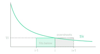
Sum the second inequality over all $i$ and the first from $i = 2$ (the $i = 1$ term is worth $1$ and is taken out separately), and the rectangles are trapped:

$$\int_{1}^{k+1} \frac{dx}{x} \;\leq\; \sum_{i=1}^{k} \frac{1}{i} \;\leq\; 1 + \int_{1}^{k} \frac{dx}{x}.$$

The two ends are worth $\ln(k+1)$ and $1 + \ln k$, so the sum is $\ln k$ plus something that stays between $0$ and $1$. That "something" converges, and its limit is the Euler-Mascheroni constant $\gamma \approx 0.577$. What the lesson uses is the part that grows: the logarithm.

And here is the result that decides the size of the vocabulary. Ask for a coverage $p$ and solve for $k$. Since $\ln M$ is around $11.5$ for a corpus with a hundred thousand types, $\gamma$ is negligible beside it and the equation $\ln k \approx p \ln M$ leaves

That exponent decides everything: coverage is not paid in proportion, it is paid in powers. With $M = 100\,000$ types, covering half the corpus costs $M^{0.5} \approx 316$ types, 90% costs $M^{0.9} \approx 31\,600$, and 99%, $M^{0.99} \approx 89\,000$. The last nine points of coverage almost triple the vocabulary.

What it costs to cut the vocabulary

The vocabulary is then a decision with two opposed prices. Choosing $V$ as the $k$ most frequent types (or, from another angle, demanding a minimum frequency $f_i \geq m$) is choosing where the trade stops.

The price of raising $k$ is set by the lesson on the problem of representing languageBlock 1 · Lesson 1The problem of representing languageA network operates only on real numbers. Text does not. This is the precise statement of the problem the whole block lives on.: the representation is a function $r : V \to \mathbb{R}^{d}$, and a function like that is stored as a table with one row per vocabulary entry and $d$ columns. That is

With $d = 300$, a vocabulary of 30,000 types is nine million numbers; one of 100,000, thirty million. The table grows with $\lvert V \rvert$ and nothing compresses it: each entry is independent of the others.

The price of lowering $k$ is the text that falls on the far side of the cut, the fraction $1 - \text{cob}(k)$ of the occurrences. Measured that way it looks small, and that is the problem: the same decision, measured over types, leaves out most of the language. With $M = 100\,000$ and $k = 31\,600$ you lose 10% of the occurrences and 68% of the types. And it is not a random 68%: the types that fall are the tail ones (proper nouns, technical terms, new words), the very thing that makes a sentence say one thing rather than another. A cut that sounds cheap in tokens is throwing away exactly the informative part.

The token that gathers what falls outside

That leaves the third question: what to do when, already in production, a word arrives that was left outside. The standard fix is to add one more entry to the vocabulary, one that corresponds to no particular word and absorbs them all, written <UNK>, for unknown:

and, before representing anything, each word passes through a filter that leaves it untouched or replaces it:

With that, $r(\tilde{w})$ is defined for any word that arrives. That was totality, the first of the three demands from that lesson on the problem of representing language, and it is the one this fix recovers. What you pay is injectivity: cryptocurrency and librarian become the same object. That lesson already warned that you would give it up on purpose, and this is the place it happens for the first time.

Now to name what it costs. The fraction of text that ends up in that entry is the OOV rate, and it is measured in the two directions this lesson has been keeping apart. Take a new text, $w_1, \dots, w_{T'}$, and call $U$ the set of its types, so that $\lvert U \rvert = M'$; the prime marks what is measured on that text and not on the original corpus. Then

On the left there are positions: if cryptocurrency appears ten times, it contributes ten. On the right there are distinct strings, and that same word contributes one. They measure the same decision and give very different numbers. In a real corpus, a reasonable vocabulary leaves an OOV rate over tokens of 2% or 3%, and one over types of 30% or 40%. The first is the one that gets quoted, because it is the one that reassures. It is also the one that misleads, and in two ways.

One is arithmetic. The rate is measured per token, but text is read by sentences, and a sentence is spared only if all its tokens are in $V$. With twenty tokens per sentence and a 2% OOV rate, that happens with probability $0.98^{20} \approx 0.67$: one in three sentences contains some word the model cannot read. The other way is that the tokens that fall are not arbitrary ones, but the tail ones, the ones carrying what the sentence says. A 2% loss of tokens is not a 2% loss of meaning.

Counting types, tokens and coverage in Python

The cell tokenises a short English corpus with the same by_words as the previous lesson, counts types and occurrences, walks the coverage, and ends by applying a cut to five sentences the corpus did not contain. Run it and look at three things: what fraction of the types appears a single time, how $\text{cob}(k)$ climbs at first and then jams, and the two OOV rates, which do not resemble each other.

Coverage climbs fast and then jams, which is the logarithmic shape seen in numbers: the first eight types cover more than a third of the corpus, and it takes fifty to reach three quarters. The tail is long and cheap to throw away, measured in occurrences.

Look carefully at the last two parts. The rate over types beats the rate over tokens in both vocabularies, exactly as the theory says, and the toy corpus exaggerates both: with 228 tokens, even the untrimmed vocabulary leaves out a third of what arrives, while a real one would bring the rate over tokens down to 2% or 3%. What does not change with size is which words fall. In the rewritten sentences the articles and prepositions still stand, and cryptocurrency, librarian, manuscripts and monastery disappear: the fourth sentence is reduced to a skeleton that no longer says anything.

A thirty-second test. Change V = set(freq) to V = {w for w, _ in freq.most_common(50)} and run again: In with a capital becomes unknown while in stays in. It is a different type, not a bug: the previous lesson already warned that cutting is not cleaning, and the price is paid here, in the count.

Test your intuition

Four questions on what you now have: what a cut costs, what coverage costs, what the unknown token recovers and what it spends, and what a small OOV rate really means.

The vocabulary is now a closed list: $k$ types chosen by frequency, plus one entry at the end that gathers everything else. That list, the $V'$ from above, we call $V$ from here on, with <UNK> as one more entry. With it, $r$ is once again defined on any text, which was the starting condition. But of $r$ we know only what it receives and what it returns. We still have to decide which concrete vector each of those $\lvert V \rvert$ entries gets, and the lesson on the problem of representing languageBlock 1 · Lesson 1The problem of representing languageA network operates only on real numbers. Text does not. This is the precise statement of the problem the whole block lives on. already said what will not do: with $d = 1$ the order of the real line invents likenesses between words that have none.

The most direct way out is to choose no likeness at all. If no vocabulary entry should sit closer to one than to the rest, give each its own axis: one dimension per entry, a one in its position and zeros elsewhere. That representation exists, it is called one-hot encoding, and it asserts nothing about the language, which is exactly what we asked of it. This lesson has now written its bill: $\lvert V \rvert$ runs to tens of thousands, and that is the dimension those vectors would have. The lesson on one-hot encoding and the curse of dimensionality looks at that bill up close.