The missing square root in attention

Self-attention is fully assembled except for one symbol. The three projections $\mathbf{Q}$, $\mathbf{K}$ and $\mathbf{V}$ have their argument, the weight matrix $\mathbf{A}$ is square ($T \times T$) because the sentence looks at itself, and the softmax by rows shares one unit out among the positions of each row. But the $\sqrt{d_k}$ in the denominator was written into the formula without any explanation of why it is there. It is the only loan still outstanding, and this lesson pays it off.

The question is sharper than it looks. Why a root, and not $d_k$ itself? And why of $d_k$, and not of $d_{\text{model}}$ or of the length of the sentence? Both are answered at once, because both depend on finding out how far a sum moves away from zero as terms are added to it. That takes no elaborate probability theory, only averaging, and the calculation starts by averaging over a finite list that can be walked through in full.

Take the crudest possible version of a query and a key, that is, of a row of $\mathbf{Q}$ and a row of $\mathbf{K}$: all their coordinates are $+1$ or $-1$. The score is then a count of agreements, because each term contributes $+1$ if the two coordinates share a sign and $-1$ if they do not. With four coordinates, three agreements and one disagreement give $3 - 1 = 2$. With four hundred, the same proportion (three hundred against one hundred) gives $200$.

What is worth noticing is not that the terms have grown, since they are still $\pm 1$, but that there are a hundred times as many of them. A small deviation from an even split, repeated over more terms, turns into a large number, and the softmax is about to exponentiate that number.

With random signs the proportion does not stay fixed at three to one, and the score grows more slowly: its typical size goes with $\sqrt{d_k}$, as the next section derives. The figure takes one row of six scores at that size in three widths and tries three divisors before the softmax: $1$ (that is, not dividing), $\sqrt{d_k}$ and $d_k$ itself. Each group of bars is the row's share-out, one weight per position, and the number above it is what the winning position takes. Look for the row that does not change from one column to the next.

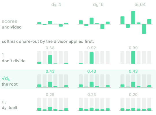
A score grows with the root of the width

Each cell of $\mathbf{Q}\mathbf{K}^{\top}$ is the dot product of a row of $\mathbf{Q}$ (the query of one position) with a row of $\mathbf{K}$ (the key of another). Both live in $\mathbb{R}^{d_k}$, and I write them $\mathbf{q}$ and $\mathbf{k}$ without a position index, because the calculation is the same for any pair. The score is

a sum of $d_k$ terms. The size that comes out depends on the size that goes in, so let's fix the exact case first: the coordinates are $+1$ or $-1$, as in the count of agreements above. Call $s_m = q_m k_m$ the $m$-th term, which is then $+1$ or $-1$, and $e = \sum_m s_m$.

Squaring separates the diagonal from the rest:

because $s_m^{2} = 1$ whatever the sign. The first term no longer depends on anything. The second is the one that has to be averaged, and averaging here means something perfectly finite: running through the $2^{d_k}$ sign combinations $\mathbf{q}$ can take, with $\mathbf{k}$ fixed, and taking the mean. We write it $\mathbb{E}\left[\cdot\right]$, the mean of a quantity over the randomness it is assumed to have. The cross terms all disappear.

So of the square, only the first term survives:

With $\mathbb{E}\left[e\right] = 0$, that is all it takes. The score is spread around zero, and what measures how far it typically lands from it (the standard deviation) is the root of that mean:

which answers half the question. Dividing by $\sqrt{d_k}$ leaves $\mathbb{E}\left[\left(e/\sqrt{d_k}\right)^{2}\right] = 1$, and $d_k$ does not appear in that $1$: the same scale for queries of eight coordinates and for queries of a thousand.

With the divisor in place, the whole operation (product, division, softmax and mixture) gets a name of its own: the scaled dot-product, which is what the paper calls it. The dot product is the ordinary one, the one in the line above; what is scaled is this division and nothing more.

The signs were there to make the calculation exact, but notice which properties it really needed. Two: that $\mathbb{E}\left[s_m\right] = 0$ and that $\mathbb{E}\left[s_m^{2}\right] = 1$. Any centred initialisation whose coordinates are independent and of typical size $1$ meets them, and with them the same cancellation leaves the same $\mathbb{E}\left[e^{2}\right] = d_k$. The Gaussians from rng.normal that the course has used since the lesson on implementing an MLPBlock 2 · Lesson 9Implementing an MLP from scratchThe four pieces of training are all derived by now, and no cell has ever run them one after another. Assembling them costs stacking the backward pass by rows (bringing along the 1/B the mean introduces) and making the one decision no formula makes: where the weights start from. Start them all equal and they stay equal forever, which is exactly why initialisation has to be random. are one such initialisation, and the first cell below measures it with them.

It is worth saying out loud what that assumption is about, because it is not about the model you will end up using. It is about a freshly initialised network: nothing guarantees that after thousands of steps the coordinates of $\mathbf{q}$ are still independent or still of size $1$. That is why the divisor is fixed when the layer is designed rather than measured on the fly: it fixes the start, which is where the problem halts training before it has even begun.

That leaves the part usually taken for granted: why the root and not $d_k$. The divisor has to take away from the score exactly what the width put into it, and what the width put in is a factor of $\sqrt{d_k}$. Dividing by $d_k$ would leave the scores at a typical size of $1/\sqrt{d_k}$, closer and closer to zero the wider the model; and scores that tend to zero give a softmax that tends to the even share, $1/T$ in every cell, so the row stops choosing anything. Those are two failures, one on each side, and the root is the only exponent that falls into neither.

A closed row returns no gradient

If the scores measure $\sqrt{d_k}$, the differences between the scores in a row measure that too, and what the softmax looks at is the differences:

with $m$ running over the positions of row $i$. Two scores $8$ apart (an ordinary gap when the typical size is $8$, which is what $d_k = 64$ gives) end up a factor $\exp(8) \approx 2\,981$ from each other, and with that the share-out is over: one position takes almost the whole unit.

A row that chooses firmly does not sound like a defect. The defect is in the derivative.

Differentiate $\alpha_{ij}$ with respect to the scores of its own row. It is the same calculation that the lesson on loss functionsBlock 2 · Lesson 5Loss functions: MSE and cross-entropyA loss sums up in one number how badly the network is doing, and between two candidates its derivative is what decides. Mean squared error hands over its smallest correction exactly where the network is wrong with the most confidence; cross-entropy, which comes from reading the output as a probability, leaves that derivative at the plain difference between what was predicted and the label. did with the softmax of the output layer, and the same two cases come out, depending on whether the indices match:

Now take the closed row, with one weight at almost $1$ and the rest at almost $0$. The diagonal case gives $1$ times $0$; the cross case, in any cell, carries at least one factor that is almost zero. Both derivatives switch off at once, and the whole row with them.

What that costs becomes clear when you look at what comes before the scores: only $\mathbf{W}^Q$ and $\mathbf{W}^K$, since the scores come out of $\mathbf{Q}\mathbf{K}^{\top}$ and nothing else goes in. If the gradient does not get through the softmax, those two matrices receive nothing from that row, and they are precisely the ones that would have to learn which positions each position should look at. The layer goes on computing (a saturated output is a perfectly well-defined output); what it can no longer do is change its mind.

It is worth pausing on why Block 2 never ran into this, because the difference is one line. There the softmax was followed by the cross-entropy, and the $-\log$ of the loss supplies the exact inverse factor: together the two gave $\nabla_{\mathbf{z}}\,\ell = \hat{\mathbf{y}} - \mathbf{y}$, which is $\hat{y}_c - 1$ in the correct class and does not vanish while the network is wrong, however sure of itself it is. Here there is no logarithm behind the softmax, only the multiplication by $\mathbf{V}$, the matrix of values. The Jacobian cancels against nothing: it stays whole, zeros included.

And so two things the course had closed, in different blocks, turn up again. The curve $\alpha\left(1 - \alpha\right)$ is the same as the derivative of the sigmoid, with its maximum of $0.25$ in the middle and its two flat tails: the saturation from the lesson on activation functionsBlock 2 · Lesson 2Activation functions and non-linearityThe step passes along the sign of the pre-activation and drops everything else, and its derivative is zero wherever it even exists. Sigmoid, hyperbolic tangent and ReLU keep the magnitude instead and have a real derivative; none of them can be a straight line, because chaining affine functions together only ever gives back another affine function., in a layer with no sigmoid in it. And a gradient that arrives switched off at the matrices that were meant to learn is the whole of Block 3, in an architecture without a single recurrence. What joined them was never the sigmoid or the recurrent state: it was that in both there was a function flattening out.

A whole row comes down to one number, which comes from adding the diagonal case over the $T$ positions:

where the last equality uses that the row sums to $1$. With the row shared out evenly it is $1 - 1/T$; with the whole row on one position it is $0$. It is the sum of the diagonal of the Jacobian, and it measures the same thing from both sides: how much that row shares out, and how much it still has left to learn.

The divisor, measured in NumPy

The first cell takes the calculation done for signs and checks it where it actually applies: Gaussian coordinates, five widths, with the measured typical size set beside the $\sqrt{d_k}$ column.

The two middle columns agree as far as a sample of eight thousand pairs allows, and the one on the right stays pinned at $1$: dividing puts the size in the same place whatever the width. The mean column is small next to the typical size on its row (at $d_k = 1\,024$, $0.236$ against $32.03$), which is what $\mathbb{E}\left[e\right] = 0$ says when it is measured instead of proved.

The second cell moves from the scores to what comes out of them. Pay particular attention to the last column, which decides whether the layer can learn.

Read it in pairs of lines. Undivided, the top weight climbs from $0.670$ to $0.953$ and the share-out $1 - \sum_j \alpha_{ij}^{2}$ sinks from $0.445$ to $0.066$ (the most it can be with eight positions is $1 - 1/8 = 0.875$), while the largest cell on the diagonal of the Jacobian falls from $0.1755$ to $0.0321$: more than five times less gradient for no reason other than having widened the model. Divided, the three lines stop moving: $0.36$ of top weight, $0.77$ of share-out and $0.216$ of derivative at all three widths, $512$ included. That is the property the divisor buys. It does not make the numbers better; it makes them stop depending on $d_k$.

Test your intuition

Five questions: how big a score is, why the root and nothing else, what a closed row loses, why Block 2 escaped this, and what dividing does not touch.

With the divisor in place, the scale of the scores stops depending on the width, and the share-out and the gradient stop depending on it by the same calculation. But look at what the divisor takes for granted: it receives $d_k$ already decided. Nothing worked out so far says how long a query should be (only how to compensate for whatever length it has), and until now $d_k$ has been a number that turned up because the projections of the previous lesson had to come out at some width.

There is a second thing this layer cannot do, and it points to the same place. A row of $\mathbf{A}$ is a share-out, and only one: in the keys to this car are here, the position of are has to decide, with a single set of weights, whether to look at keys, which is what it agrees with, or at to this car, which is what stands between them; and with one row it cannot do both. The answer to both questions is the same and takes up the next lesson, on multi-head attention: several pairs of projections working in parallel, each with its own share-out and its own width, carved out of $d_{\text{model}}$. There, $d_k$ stops being a given number and becomes a decision with a reason.