One-hot encoding and the curse of dimensionality

22 min read

The previous lesson, on vocabulary and frequency, left the vocabulary completely defined: a closed list of $\lvert V \rvert$ entries, built from the most frequent words and rounded out with <UNK> for everything that falls outside. With that, $r$ can now accept any text. All that remains is to decide which vector to assign to each of the vocabulary entries.

There is an immediate answer to that question, and the lesson exists because that answer is correct: it meets, one by one, the demands the lesson on the problem of representing language placed on $r$ , and still it is not enough. It has a name, one-hot encoding, and what remains to be done with it is to put a price on it. Part of the price is visible from the outset, because the vectors come out enormous, and it is precisely the part that does not matter. The other part shows up when you ask what a model can learn from inputs like these, and no larger machine will fix that one.

Look at the three words that lesson used to rule out $d = 1$ , laid out both ways, before you read a single formula. On the line, the indices $1$ , $2$ and $3$ leave cat at distance $1$ from apple and dog at distance $2$ : there is a middle, and one of them sits in it. With one axis per word there are three perpendicular axes and each word falls on its own, at $(1,0,0)$ , $(0,1,0)$ and $(0,0,1)$ . Count the distinct side lengths of the triangle they form.

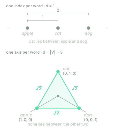
Above, apple, cat and dog on a line with the indices 1, 2 and 3: cat is at distance 1 from apple and dog is at distance 2, so cat lies between the other two. Below, the same three words in a space with three perpendicular axes, one on each axis, at the points (1,0,0), (0,1,0) and (0,0,1); the three points form an equilateral triangle whose sides measure root 2. — The same three words, two representations. On the line there is one word in the middle; with one axis per word each of them goes to its own axis and the three end up at the same distance from each other.

One axis for each vocabulary entry

Order the vocabulary once and for all and write it as $V = \{w_1, w_2, \dots, w_{\lvert V \rvert}\}$ . The order doesn't matter (alphabetical, by frequency, whichever) as long as it doesn't change afterwards; it is the determinism the lesson on the problem of representing language demanded. What that order contributes is a correspondence: the entry in position $i$ has coordinate $i$ of the vector reserved for it, and no other entry uses that coordinate. Vocabulary positions and vector coordinates are, from here on, the same list of numbers from $1$ to $\lvert V \rvert$ .

One thing still needs saying: what that list is made of, because the rest of the lesson takes it for granted. The entries of $V$ are tokens, and what they are depends on the tokenisation fixed by the lesson on tokenisation: whole words with a word tokeniser, word-pieces with a subword one. Nothing that follows changes because of it, and the examples use whole words because they read better.

The one-hot representation assigns to the entry $w_i$ the vector of $\lvert V \rvert$ coordinates that is $1$ at position $i$ and $0$ everywhere else. Coordinate by coordinate, writing $(\mathbf{o}_w)_j$ for the $j$ -th coordinate of the vector of the entry $w$ :

\mathbf{o}_{w_i} \in \{0,1\}^{\lvert V \rvert}, \qquad (\mathbf{o}_{w_i})_j = \begin{cases} 1 & \text{if } j = i \\ 0 & \text{if } j \neq i \end{cases}.

It is an $r$ like the one the lesson on the problem of representing language asked for, with the dimension fixed by the vocabulary itself: $r(w) = \mathbf{o}_w$ and $d = \lvert V \rvert$ . A text of $T$ tokens then turns into a matrix $\mathbf{X} \in \mathbb{R}^{T \times \lvert V \rvert}$ , one row per position.

Now the property it is chosen for. Take two distinct vocabulary entries, $u$ at position $i$ and $v$ at position $j$ , with $i \neq j$ . Their dot product runs through the coordinates $k$ and hits a zero at every one:

\mathbf{o}_u^{\top} \mathbf{o}_v = \sum_{k=1}^{\lvert V \rvert} (\mathbf{o}_u)_k \, (\mathbf{o}_v)_k = 0,

because the only term that could fail to vanish would need $k = i$ and $k = j$ at once. The vectors are orthogonal, in pairs, all of them.

And the distance between them comes out of the same sum. We write it with a double bar: $\lVert \mathbf{x} \rVert$ is the Euclidean length of $\mathbf{x}$ , the root of the sum of its squared coordinates. The difference $\mathbf{o}_u - \mathbf{o}_v$ is worth $+1$ at position $i$ , $-1$ at position $j$ and $0$ everywhere else, so that

\lVert \mathbf{o}_u - \mathbf{o}_v \rVert^{2} = \sum_{k=1}^{\lvert V \rvert} \big( (\mathbf{o}_u)_k - (\mathbf{o}_v)_k \big)^{2} = 1^{2} + (-1)^{2} = 2,

and therefore $\lVert \mathbf{o}_u - \mathbf{o}_v \rVert = \sqrt{2}$ , whatever $u$ and $v$ are, and whatever the size of the vocabulary. There it is, in one line: every pair of words is at exactly the same distance. No word sits between any other two, and nothing the representation says about the language can be read wrong, because it says nothing. The invented geometry of the lesson on the problem of representing language has disappeared.

Why the dimensions are |V| and not |V| − 1

That lesson ended with a count: $n$ mutually equidistant points need $n - 1$ dimensions. The minimum is then $\lvert V \rvert - 1$ dimensions (the triangle above, with three words, fits in a plane), and one-hot spends one more. It is no oversight, and the difference shows up when you look at where these vectors live.

They all satisfy the same equation, because each has a single $1$ :

\sum_{j=1}^{\lvert V \rvert} (\mathbf{o}_w)_j = 1.

That is a hyperplane of $\mathbb{R}^{\lvert V \rvert}$ , and a hyperplane has one dimension fewer than the space that contains it: the $\lvert V \rvert$ vertices in fact live in $\lvert V \rvert - 1$ dimensions, which is the minimum. What you buy with the spare dimension is that the coordinates are readable. Inside the hyperplane they would be combinations with no meaning of their own; in $\mathbb{R}^{\lvert V \rvert}$ , coordinate $j$ answers "is this the word $w_j$ ?", and that is why representing a word means looking at a position rather than computing anything.

What asserting nothing costs

The price was already written in the previous lesson, only the substitution was left to make. Storing $r$ as a table, one row per vocabulary entry and $d$ columns, costs $\lvert V \rvert \cdot d$ numbers; with $d = \lvert V \rvert$ that is

\lvert V \rvert^{2} \quad \text{numbers}.

With the subword vocabulary of the lesson on tokenisation, between 30,000 and 50,000 entries, that is between 900 million and 2.5 billion numbers: about 10 GB with four bytes each. And it grows as the square: doubling the vocabulary quadruples the table.

That figure calls for an immediate correction, because nobody pays those 10 GB. The one-hot table is the identity matrix, and an identity matrix carries no information: it is determined by its size. The index $i$ of each entry gets stored (an integer), and the vector is built when it is needed, or not built at all. The cost of storing the representation disappears.

What does not disappear is the dimension. The vector the system receives has $\lvert V \rvert$ coordinates and only one of them is nonzero, so the part of the vector that carries information, with 50,000 entries, is

\frac{\text{nonzero coordinates}}{\text{coordinates of the vector}} = \frac{1}{\lvert V \rvert} = \frac{1}{50\,000} = 0.00002 = 0.002\ \%.

Before going on, a point in one-hot's favour. The lesson on the problem of representing language told you to hold on to an observation: there, adding bird to the vocabulary renumbered words that had nothing to do with it and left any model trained beforehand useless. One-hot doesn't have that flaw. Add an entry at the end and every old vector keeps its coordinates; only a zero is appended. It is the stability that was missing. It is real, though in practice $V$ is frozen once and for all (that is what <UNK> is for), and the occasion barely comes up.

Why orthogonality prevents learning

The count that gives the lesson its title is still to come, and it is not the one about memory. A system reading a window of $n$ consecutive tokens receives the $n$ vectors one after another, $n \lvert V \rvert$ coordinates in all. How many distinct inputs can it receive? Each of the $n$ positions admits any of the $\lvert V \rvert$ vocabulary entries, independently of the others, so

\lvert V \rvert^{n}.

Plug in small numbers: $\lvert V \rvert = 30\,000$ and a window of $n = 5$ tokens, a quarter of the twenty-token sentence from the lesson on vocabulary and frequency. That is $30\,000^{5} \approx 2.4 \times 10^{22}$ possible inputs. A huge corpus is of the order of $T = 10^{10}$ tokens, and therefore holds at most $10^{10}$ distinct windows, so the model gets to see

\frac{10^{10}}{2.4 \times 10^{22}} \approx 4 \times 10^{-13}

of the input space. Four ten-millionths of a millionth. And no corpus fixes it: the exponent is in $n$ , so looking at one more token of context multiplies the space by $30\,000$ while the corpus stays where it was. This is the curse of dimensionality: the number of distinct configurations grows exponentially with the dimension of the input, and any amount of data covers a fraction that tends to zero.

Put that way it sounds like a general condemnation, and it isn't. Models work with enormous-dimensional inputs and learn anyway, because those inputs have neighbourhoods: two photographs differing in one pixel are alike, what is learned about one holds for the other, and that is why a minute fraction of the space is enough. That is the argument that saves any high-dimensional representation, and it is the one one-hot cannot use. The equidistance worked out above says, in other words, that here there are no neighbours: the window the boy plays in the square and the window the girl plays in the square are at the same distance from each other as from anything else.

So the virtue is the flaw, and it is the same property seen twice. We asked for a representation that would not assert false likenesses, and what we got asserts no likenesses whatsoever. Each of those $2.4 \times 10^{22}$ inputs has to be learned separately, because none is like any other, and only $10^{10}$ will ever be seen.

The one-hot matrix in NumPy, and how much space it would take

The cell builds the one-hot of a tiny English vocabulary and checks the three claims from above against it: that the vectors are orthogonal, that every distance is $\sqrt{2}$ and what fraction of each vector is nonzero. Then it does the size counts without allocating memory, which is the only way to do them: a 50,000 by 50,000 table does not fit in the browser, and that is part of the result.

import numpy as np

V = ["<UNK>", "of", "the", "boy", "girl", "school", "programming", "river"]
n = len(V)

O = np.eye(n, dtype=int)          # row i = one-hot vector of V[i]
print("|V| =", n, " ->  O has shape", O.shape)
print(O)
print()

# Orthogonality: the matrix times its transpose is the identity,
# i.e. every dot product between distinct vectors is 0.
print("O @ O.T == identity:", np.array_equal(O @ O.T, np.eye(n, dtype=int)))

# Every pairwise distance is the same, and that same value is root 2.
distances = set()
for i in range(n):
  for j in range(i + 1, n):
      distances.add(round(float(np.linalg.norm(O[i] - O[j])), 6))
print("distinct pairwise distances:", distances, " |  sqrt(2) =", round(float(np.sqrt(2)), 6))
print("nonzeros per vector:", int((O[3] != 0).sum()), "of", n,
    "->", round(100 / n, 3), "%")
print()

# The explicit table: |V| x |V| numbers. Computed, NOT allocated.
print(" |V|        numbers        GB (4 bytes)   % nonzero")
for size in [8, 1000, 30000, 50000]:
  numbers = size * size
  gb = numbers * 4 / 1024**3
  print(str(size).rjust(6), str(numbers).rjust(15), ("%.2f" % gb).rjust(13),
        ("%.5f" % (100 / size)).rjust(11))
print()

# The space of inputs for a window of n tokens, against a large corpus.
T = 10**10                        # tokens of a huge corpus
size = 30000
for window in [1, 2, 3, 5]:
  possible = size ** window
  covered = min(T, possible) / possible
  print("n =", window, "->", ("%.1e" % possible).rjust(8),
        "possible windows  |  fraction covered by corpus:", "%.1e" % covered)

numpy

The first run downloads the Python interpreter (~15 MB). After that it stays in the browser cache and is reused across every lesson.

The three checks come out exactly and one is worth looking at twice: the set of pairwise distances has a single element. It is not that they are close to one another; there is only one value. With eight words you see it at a glance; with 50,000 it is still the problem.

The size table has one surprising row and one that isn't. The unsurprising one: 50,000 entries take 9.31 GB, and that is why nobody stores this table. The surprising one: the right-hand column, the percentage of nonzero coordinates, which is already 0.003 % at 30,000 entries. And the last lines are the curse of dimensionality in four rows: with one or two words of context the corpus covers the whole space, with three it covers only 0.04 %, and with five the fraction is written with twelve zeros after the point. The jump happens between the second and third context word, not out at infinity.

A thirty-second test. Change V to a two-word vocabulary and run it again: the pairwise distance is still $\sqrt{2}$ , exactly as with eight. That is where you see that $\lvert V \rvert$ does not enter the sum.

Test your intuition

Four questions on what you now have: how large the distance between two words is, what one-hot fixes relative to the lesson on the problem of representing language, what the table costs, and what happens to two words that look alike.

Your vocabulary has $\lvert V \rvert = 20\,000$ entries and you represent each with its one-hot vector. What is the Euclidean distance $\lVert \mathbf{o}_u - \mathbf{o}_v \rVert$ between the vectors of two distinct entries $u$ and $v$ ?

A margin of ±0.01 is accepted.

You compare one-hot with the index representation from the lesson on the problem of representing language. Where does it improve? Tick all that apply.

Select every correct option. This is graded all-or-nothing: there is no partial credit.

It doesn't assert likenesses nobody meant to assert: no vocabulary entry sits between any other two.It's stable: adding an entry at the end leaves the coordinates of every other entry untouched.By not asserting false likenesses, the model generalises better from one word to another.It recovers totality on its own: the <UNK> entry is no longer needed.

With $\lvert V \rvert = 50\,000$ , how many numbers would a table storing $r$ explicitly hold, one row per vocabulary entry?

50,000, one per entry.2.5 billion:

\lvert V \rvert

rows of

\lvert V \rvert

columns.15 million:

\lvert V \rvert \cdot 300

, the usual dimension.You can't tell without knowing the corpus.

A model trained on one-hot vectors has seen the boy plays many times and the girl plays not once. What it has learned about boy helps it a little with girl, because the two words are similar.

TrueFalse

One-hot meets the three demands, is stable, and its geometry asserts nothing false about the language. It is also a dead end, and a dead end for the very reason it works: a representation that relates no word to any other forces you to learn everything separately, and there is no corpus for that. Getting out of it needs two things at once, and they are the two that are missing here: many fewer coordinates than $\lvert V \rvert$ , and coordinates that mean something, so that two similar words end up close.

The second is the hard one and occupies the rest of the block. But before that there is a change of question that comes almost for free from here, and it is worth making now, with the one-hot vectors still in view. Up to now $r$ represents one word, and what a system usually needs is the vector of a whole document: a review, an email, a news article. The most direct way to obtain it is to sum the one-hot vectors of all its tokens, $\sum_{t=1}^{T} \mathbf{o}_{w_t}$ , where $t$ runs over the $T$ positions of the document and not over the vocabulary entries. Each coordinate then comes to count how many times its word appears. That is no longer a vector of zeros and ones, and no longer as silent: the coordinate of goal tells a match report from a recipe. It still has $\lvert V \rvert$ dimensions and it still doesn't know in what order the words came. It is the bag of words, and with the correction that makes it useful, TF-IDF, it is the lesson on the bag of words and TF-IDF.