How a vector database searches without comparing everything, and the price it pays

You have a million passages of text, and each one has been turned into an embedding: a vector of 768 numbers that a model uses to represent what the passage says, trained so that two texts with similar meanings get nearby vectors. A query arrives, it's turned into a vector of the same kind, and you have to return the ten passages whose vectors are closest to it. That's what a semantic search engine does, and so does the search half of a RAG system (retrieval-augmented generation: finding passages and handing them to a language model so it can answer from them), a song recommender or a search for similar photos.

The safe way to do it is to compare the query with all million. That's 768 million multiplications per query over 3 GB of vectors, and on a single core of a processor it takes a few tenths of a second. (A core is one of the units in a processor that execute instructions independently; a laptop has a few and a server has dozens.) For an occasional query, that's fine. For a hundred per second, or for a billion vectors, it isn't.

In a relational database, a problem like this is solved with an index, almost always a B-tree, which finds one row among millions by reading three or four blocks from disk. But a B-tree needs its keys to have an order, and vectors don't have one: there's no way to line up a million points in 768 dimensions so that the nearby ones end up together. You need a different kind of index, and the kind vector databases use differs from the ones you know in something fundamental: it's approximate. It doesn't promise to find the ten nearest. It promises to almost always find almost all of them, and it lets you choose how much "almost" you'll accept in exchange for how much speed.

This article goes through how those indexes are built: the four families of algorithms that decide where to look, the compression techniques that decide how much of each vector to keep, how the two combine in the indexes actually in use, what databases have had to add on top, and how everything compares. The performance numbers come from two public benchmarks; they're cited here, not measured.

What a vector database is, and what it isn't

A vector database stores, for each object, a vector, an identifier and almost always a few more fields: the original text, the date, the language, the customer it belongs to. Its core operation is just one: given a vector and a number $k$ , return the $k$ objects whose vectors are closest. The objects don't have to be documents. They can be passages of text, images, songs, products or users, anything a model knows how to assign a vector to.

People often say a vector database is NoSQL, and that's true only in the weakest sense of the word. NoSQL covers everything that isn't relational, lumping together key-value, document, column and graph stores, which differ from one another in how they model data. What defines a vector database isn't how it models data but how it searches it. Milvus, Qdrant, Weaviate, Pinecone and Chroma are dedicated databases, built around that search. But the same search now exists as one more feature inside databases of every family: in PostgreSQL through the pgvector extension, in Oracle, in SQL Server 2025, in MongoDB Atlas, in Elasticsearch and in Redis. "Vector database" has ended up naming a capability more than a family.

A second idea worth correcting early is the order in which things happened. The algorithms these databases use weren't invented for them. The k-d tree dates from 1975; locality-sensitive hashing, from 1998; product quantization, from 2011; HNSW, the graph index almost all of them use today, from 2016. They were born in computational geometry, image search and recommender systems, and were published as programming libraries: Annoy, from Spotify, in 2013; Faiss, from Facebook, in 2017. The dedicated databases came later, from 2019 on, and Milvus was built directly on top of Faiss. What the databases did contribute were variants: ways to filter while searching, to insert and delete without rebuilding the index, and to keep the index from having to fit in memory.

Timeline, not to scale, in two rows. Above, in green, algorithms and libraries: 1975, the k-d tree; 1998, locality-sensitive hashing; 2003, Video Google's inverted lists; 2011, product quantization; 2013, Annoy; 2014, NSW; 2016, HNSW; 2017, Faiss; 2019, DiskANN and NSG; 2020, ScaNN; 2021, SPANN and FreshDiskANN; 2023, Filtered-DiskANN; 2024, RaBitQ and ACORN. Below, in orange, databases: 2019, Milvus and Qdrant's filterable HNSW; 2021, pgvector; 2023, HNSW in pgvector; 2024, pgvector's iterative scans and ACORN in Weaviate; 2025, DiskANN in SQL Server. 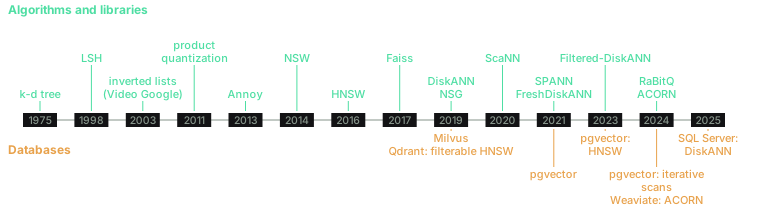— Not to scale. In green, the algorithms and the libraries; in orange, the databases and what they added.

Finding the nearest, without approximating

Before approximating, it's worth seeing why exactness isn't enough. Exact search for the $k$ nearest neighbours (k-nearest neighbors, k-NN) by brute force compares the query with every vector. With Euclidean distance or with the cosine, each comparison costs $d$ multiplications and $d$ additions, so the total cost grows with the number of vectors times their dimension. What makes it slow isn't the arithmetic, which a processor does many operations at a time with vector instructions, but the memory: a million vectors of 768 four-byte numbers take up 3 GB, and every query has to read all of it. In ANN-Benchmarks, the reference public benchmark for years, brute force over a million 960-dimensional vectors answers 2.6 queries per second: almost 0.4 seconds per query. That's what a single core of a third-generation Intel Xeon achieves on an Amazon Web Services server (an r6i.16xlarge instance).

Brute force has virtues the rest of this article will make us miss. It's exact, there's nothing to build, it accepts any filter and it doesn't mind the data changing. The Faiss guide for Meta's vector search library says it bluntly: the only index that guarantees exact results is the flat one, the one that compares against everything. With a few tens of thousands of vectors, or with a GPU, it's often enough.

To do better than brute force, the classic idea is to partition the space. The k-d tree (k-dimensional tree), which Jon Bentley published in 1975, splits the set of points in two at the median of one coordinate. You take every value of that coordinate, the first one for example, compute the median, and the points whose first coordinate is below the median go into one group and the rest into the other. Then each half is split in two by another coordinate, and so on until the leaves are small (with few points). To search, you go down to the leaf where the query would fall, take the best candidate in that leaf (the closest one) and then climb back up, checking the branches that could still hold something closer. In two or three dimensions, this discards almost the whole tree without looking at it.

In 768 dimensions it discards almost nothing. A tree over a million points has about twenty levels, so the path from the root to a leaf decides using only twenty of the 768 coordinates. The nearest neighbour differs slightly from the query in every coordinate, and all it takes is for it to sit on the other side of just one of those twenty cuts for the search to have to double back. With so many coordinates and so small a difference in each, it will sit on the other side of many of them, and doubling back ends up visiting almost every leaf.

The problem was known long before embeddings and vector databases. In the late nineties people were already searching for similar images by describing each one with a vector, for example a colour histogram (how many pixels of each shade the image has) with hundreds of dimensions, and indexing those vectors with trees that partition the space into regions, such as the k-d tree. In 1998, Roger Weber, Hans-Jörg Schek and Stephen Blott analysed that family of trees and proved that, above about ten dimensions, reading all the data sequentially wins on average.

So what's left is to give up on exactness. An approximate nearest neighbours index (approximate nearest neighbors, ANN) returns $k$ vectors that almost always match the true $k$ almost entirely. The measure of that "almost" is recall, the fraction of the true neighbours that appear in the answer:

\text{recall@}k = \frac{\lvert \text{returned} \cap \text{true} \rvert}{k}.

A recall@10 of $0.95$ means that, out of every ten true neighbours, the answer contains nine and a half on average. And recall isn't a fixed property of the index. Almost all indexes have a parameter that's set at query time and trades speed for recall without rebuilding anything, so the results of any serious comparison are curves: queries per second against recall.

Two decisions: where to look and how much to keep

Every approximate index makes the same deal, and it's easier to understand when split into two independent decisions, because real indexes combine one answer to each.

The first is where to look: how to pick, for each query, a small fraction of the vectors worth comparing against, without comparing against the rest. There are four families of answers: partitioning the space with trees, grouping with hash functions, grouping by proximity into lists, or linking the vectors into a graph and walking it.

The second is how much to keep of each vector: whether comparisons are made with the 768 floating-point numbers or with a compressed version that takes up a fraction of the space and compares faster, at the cost of some error.

The first decision saves comparisons. The second makes each comparison cheaper and, above all, lets the index fit in memory. Both are paid for in recall.

Where to look

To compare the families with data, I use the results of VIBE (Vector Index Benchmark for Embeddings), a benchmark published in 2025 by researchers from the universities of Helsinki, Aalto and Padua and from the IT University of Copenhagen. One of its datasets is exactly this article's case: 1,344,643 abstracts of arXiv papers turned into 768-dimensional vectors, 4.1 GB in floating point. Each index is tested on a single core of a server with two Intel Xeon Gold 6230 processors, across many configurations, measuring how many queries per second it answers and with what recall@100. For each family I quote its best configuration with a recall of at least $0.95$ ; the full comparison comes further down.

Random trees

The k-d tree fails because it cuts along coordinates. Annoy (Approximate Nearest Neighbors Oh Yeah), the library Erik Bernhardsson wrote at Spotify to recommend music, cuts along random planes instead: at each node it picks two random points and splits the space with the plane equidistant from both. And instead of one tree it builds a forest of hundreds, each with different cuts. A neighbour that ends up on the other side of a cut in one tree lies on the same side in others, so searching them all at once, with a shared budget of nodes to visit, recovers what each tree on its own would miss.

It works, but every extra tree is another whole structure in memory. In VIBE, Annoy needs 12 GB to index 4.1 GB of vectors, and answers 117 queries per second. On top of that, an Annoy index doesn't accept anything new once it's built.

Hashing: making similar things collide

An ordinary hash function scatters keys at random, and two almost identical keys end up in different buckets. Locality-sensitive hashing (LSH), which Piotr Indyk and Rajeev Motwani proposed in 1998, seeks the opposite: functions under which two nearby vectors fall into the same bucket with much higher probability than two distant ones. To search, you compute the query's bucket and compare only with what's inside.

For the cosine there's a very simple function of this kind, SimHash, by Moses Charikar (2002). You pick a random plane through the origin, and a vector's hash is a single bit: which side of the plane it falls on. Two vectors get the same bit unless the plane passes between them, and that happens with a probability proportional to the angle $\theta$ between them:

P\big[h(a) = h(b)\big] = 1 - \frac{\theta}{\pi}.

A circle with two vectors, a and b, thirty degrees apart, and six random lines through the centre. The only line inside the angle between a and b, in orange, separates them and gives them different bits; the others, in grey, leave them on the same side. On the right, the arithmetic: a random line falls inside the angle with probability theta over pi, so two vectors thirty degrees apart get the same bit with probability 0.83, and two perpendicular ones with 0.50. With 10-bit keys and 20 tables, a vector at 30 degrees comes out as a candidate 97% of the time; at 60 degrees, 30%; at 90 degrees, 2%. 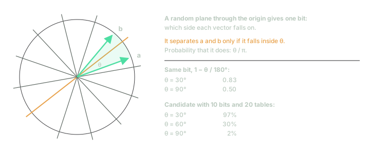— A random plane separates a and b only if it falls inside the angle between them: probability $\theta/\pi$ .

One bit separates little. Two vectors 30° apart share a bit with probability $0.83$ , and two perpendicular ones with $0.5$ . That's why $b$ planes are concatenated into a $b$ -bit key, which matches in full with probability $(1 - \theta/\pi)^b$ , and $L$ independent tables are built so that matching in any one of them is enough. The probability that a vector at angle $\theta$ from the query comes out as a candidate is

1 - \Big(1 - \big(1 - \tfrac{\theta}{\pi}\big)^{b}\Big)^{L}.

With $b = 10$ and $L = 20$ , a vector 30° from the query comes out as a candidate 97% of the time; one at 60°, 30%; a perpendicular one, 2%. It separates near from far very well, with a guarantee that can be proved, and that's its appeal.

The problem is that searching isn't about separating near from far but about ordering what's near. A query's ten neighbours and the next hundred are at similar angles, and telling them apart takes longer keys, which leave almost every bucket empty, and therefore many more tables, each with one entry per vector. That's where the memory goes. In VIBE, PUFFINN, a modern LSH implementation, takes up 9.5 GB and answers 12 queries per second: the last of all the families.

Inverted lists: cluster, then visit the nearby clusters

The third idea comes from text search engines, which store, for each word, the list of documents that contain it: an inverted index. In 2003, Josef Sivic and Andrew Zisserman brought it to vectors in Video Google, a system for finding objects in videos. They clustered the vectors with k-means, treated each cluster as if it were a word and searched with an inverted index. Hence the name the technique still carries: IVF, for inverted file.

k-means is the most common clustering algorithm: it places $n_\text{list}$ centres and moves them until each one is the mean of the vectors closest to it. Each centre defines a cell, the region of space closer to it than to any other, and the index stores one list per cell, holding its vectors. To search, you compare the query with the $n_\text{list}$ centres, pick the $n_\text{probe}$ nearest cells and compare only with the vectors in their lists.

With a million vectors and a thousand cells, which is what pgvector recommends to start with (rows divided by a thousand), each list holds about a thousand vectors. If you visit 32 cells, the square root of a thousand, which is its other recommendation, a query makes $1{,}000 + 32 \cdot 1{,}000 = 33{,}000$ comparisons instead of a million, about thirty times fewer.

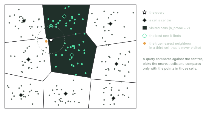
With $n_\text{probe} = 2$ the two cells with the nearest centres are visited, and the true nearest neighbour is in a third.

What gets lost is at the borders. The nearest neighbour can sit just across the border of a cell that wasn't visited, and then it doesn't show up. Raising $n_\text{probe}$ fixes this, at a cost in time proportional to the increase.

IVF has two virtues the next family lacks: it builds fast, because k-means on a sample is cheap, and inserting is trivial, because the vector just goes into the list of its nearest centre. It has one flaw: the centres were computed from the data you had at the start. If new data looks very different from the old, the lists become unbalanced and have to be recomputed, which is why pgvector asks you to create its IVF index once the table already has data. In VIBE, Faiss's IVF answers 246 queries per second and builds in under ten minutes.

Graphs: hopping from neighbour to neighbour

The fourth family is the one that won. The idea is to link each vector to a few of its neighbours and search by walking: you start at any vector, check which of its neighbours is closest to the query, hop to it, and repeat until none of the current vector's neighbours is closer than it is. It's a greedy search: each step takes the best local option.

For this to work, the graph needs two kinds of links. The short ones, between true neighbours, provide precision at the end. The long ones let you cross the space in a few hops at the start. A graph with that mix is a navigable small world (NSW): small, because any pair of nodes is only a few hops apart, as in the six degrees of separation between any two people; navigable, because those few hops can be found using local information, without knowing the whole graph. Yury Malkov and his co-authors published an index like that in 2014, in which the long links appeared on their own: vectors are inserted one by one and linked to their nearest neighbours at that moment, so the first ones, inserted when there were few, end up with distant neighbours.

In 2016, Malkov and Dmitry Yashunin separated the two kinds of links into layers, and HNSW (hierarchical navigable small world) was born. When a vector is inserted, it gets a random level, with a probability that falls off exponentially: all vectors are in layer 0, a fraction are also in layer 1, a fraction of that fraction in layer 2, and so on. Each layer is a neighbour graph among the vectors that reach it, and since the upper layers have few vectors, their links are long. The search starts in the top layer, moves greedily until it can't get any closer, drops to the next layer from that same vector and repeats. It's the idea of the skip list, a sorted list with shortcuts for skipping stretches, carried over to a space that has no order.

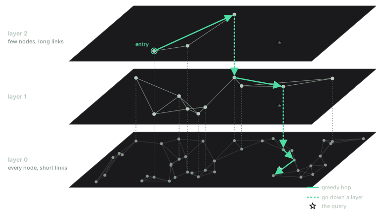
The search crosses the space with a few long hops at the top and finishes with short steps at the bottom.

In layer 0, instead of a single candidate, the search keeps a list of the $ef$ best found so far and explores the neighbours of all of them, which protects it from getting stuck in a dead end. That $ef$ is the parameter set at query time that trades speed for recall. The other two are set at build time: $M$ , how many neighbours each vector keeps (twice as many in layer 0), and $ef_\text{construction}$ , how hard each insertion searches when choosing them. pgvector's defaults are $M = 16$ , $ef_\text{construction} = 64$ and $ef_\text{search} = 40$ . The cost of a search grows with the logarithm of the number of vectors, and in VIBE the HNSW in hnswlib answers 2,001 queries per second, eight times more than the inverted lists.

It pays for that in three ways. The first is memory: on top of the vectors, about $2M$ four-byte links per vector, and everything has to be in memory, because the search jumps from one vector to another in no particular order, and on disk every hop would be a random read. The second is building, which is slow because every insertion is a search: 52 minutes in VIBE. The third is deleting, because removing a node breaks the paths that went through it; Faiss's HNSW simply doesn't support deletion.

After HNSW came single-layer graphs built with more care. NSG (navigating spreading-out graph, 2019) ended up in the search engine of Taobao, Alibaba's online shop. Vamana (2019), DiskANN's graph, deliberately keeps some long links when choosing each vector's neighbours, so it can get anywhere in fewer hops.

How much to keep: compressing to compare faster

A vector of 768 floating-point numbers takes up 3,072 bytes. A million of them take 3 GB; a hundred million, 307 GB, more than fits in the memory of almost any server. Compressing them tackles two problems at once: the index fits in memory, and each comparison reads fewer bytes, which is what really made it slow.

Scalar quantization. Each number is stored in one byte instead of four: you look at the range each coordinate moves in and split that interval into 256 steps. The vector drops to 768 bytes, four times smaller, and the error is small.

Binary quantization. Each number is reduced to its sign, one bit. The vector drops to 96 bytes, thirty-two times smaller, and comparing two vectors becomes counting how many bits they differ in (the Hamming distance), which a processor does with two instructions per 64 bits. It's the random plane from LSH, except that the planes are the axes. In Hugging Face's tests with text embedding models, searching with binary vectors keeps around 92.5% of the original search quality, and 96% if the candidates are then reranked with the uncompressed query.

Product quantization (PQ), by Hervé Jégou, Matthijs Douze and Cordelia Schmid (2011), is the most important of the three. The vector is split into $m$ consecutive chunks, for example 96 chunks of 8 numbers. For each position, a k-means with 256 centres is trained on that position's chunks from every vector; those centres are the position's codebook. Each chunk is replaced by the number of its nearest centre, which fits in a byte. The whole vector ends up in 96 bytes, and the codebooks, shared by every vector, take up $96 \cdot 256 \cdot 8$ numbers, about 786 KB.

Top: a vector of 768 numbers drawn as a strip split into 96 chunks of 8 numbers. Each chunk is replaced by the number of its nearest centre among the 256 in its codebook, one byte: 17, 203, 88 and, in the last one, 41. The vector becomes a 96-byte code, against the 3,072 bytes of the full vector. Bottom: the query, uncompressed, split into the same 96 chunks; for each chunk its distance to the 256 centres of that position is computed once, which fills a table of 96 rows and 256 columns. The distance to a stored vector is the sum of one cell per row, the one each byte of its code points to: column 17 of row 1, 203 of row 2, 88 of row 3 and so on up to 41 of row 96. 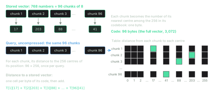— Each chunk of the vector is stored as one byte. To compare, the query fills a table once and each vector costs 96 lookups in that table.

The clever part is how it compares. The query isn't compressed. It's split into the same 96 chunks and, for each position, its distance to that position's 256 centres is computed just once, giving a table of $96 \times 256$ distances. After that, the approximate distance to any stored vector is the sum of 96 cells of that table, one for each byte of its code:

\tilde d(x, y)^2 = \sum_{j=1}^{m} \big\lVert u_j(x) - q_j\big(u_j(y)\big) \big\rVert^2 ,

where $u_j(x)$ is chunk $j$ of the query and $q_j\big(u_j(y)\big)$ is the centre that replaces chunk $j$ of the stored vector. The authors call it the asymmetric distance (asymmetric distance computation, ADC), because one side is compressed and the other isn't, and it's more precise than compressing both. It comes down to 96 additions of values read from a table that fits in the processor's cache, instead of 768 multiplications on data that has to be fetched from memory.

In 2024, Jianyang Gao and Cheng Long published RaBitQ, which also compresses each dimension into one bit, but only after rotating the vectors at random, and with a proven bound on the distance error, which PQ lacks. In their tests it beats PQ on precision for a given speed.

All compression is paid for in error, and the way to pay less is to rerank: use the compressed codes to pick a few hundred candidates quickly and compute the exact distance only for those, using the full vectors, which can live on disk because few are read. Almost every index that uses compression does this.

Real indexes are combinations

With the two decisions kept apart, the indexes that libraries and databases offer can be read as combinations.

IVF-Flat: inverted lists with the full vectors. It's pgvector's ivfflat.
IVF-PQ: inverted lists with PQ codes, the design from the 2011 paper, which tested it on two billion vectors. It's Faiss's workhorse at scale, on GPU too.
HNSW with quantization: the graph is walked comparing compressed vectors, and the finalists are reranked with the full ones.
ScaNN, from Google (2020): inverted lists, a quantization that penalises more heavily the error along the vector's own direction, since that's the error that most changes the dot product with the queries that find it, and reranking.
DiskANN (2019): the Vamana graph and the full vectors on an SSD, with only the PQ codes in memory. The codes guide the search, and each hop reads a node's neighbour list from disk together with its full vector, stored side by side so that it takes a single read. That way it indexes a billion vectors on a machine with 64 GB of memory and answers more than 5,000 queries per second, with an average latency under 3 milliseconds.

Faiss makes the idea explicit: its indexes are described with a string that names each piece. IVF65536_HNSW32,PQ32 means 65,536 inverted lists whose centres are in turn searched with a 32-neighbour HNSW graph, and vectors compressed with PQ into 32 bytes. The list part of that string is what its guide recommends for between one and ten million vectors.

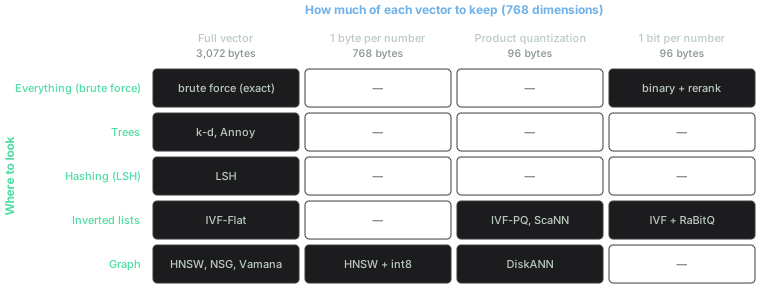
This article's indexes, each in the combination it chooses. The empty cells are combinations that are rarely used or that the article doesn't cover.

All of this fits in a library, and for years that was all there was: Annoy, Faiss, hnswlib, and later ScaNN and DiskANN. A library takes a matrix of vectors, builds the index in memory and answers queries. When the Milvus team presented their system at SIGMOD 2021, the main database conference, they explained why that wasn't enough with a list of shortcomings: libraries assume the data and the index fit in one machine's memory; they assume the data doesn't change after building; they don't support queries beyond the nearest neighbour, such as filtering by an attribute; and they don't use the processor and the GPU together. Milvus was built on top of Faiss to cover them, and the next section is, almost point by point, that list.

What a database had to add

The Big-ANN competition, organised by several of the authors of this article's indexes, has tracked that same list. Its 2021 edition tested indexes for a billion vectors with little memory or with an SSD, and its 2023 edition devoted one track each to filters, changing data, sparse vectors and queries that don't look like the data.

Filtering while searching

The typical query isn't "the ten most similar passages" but "the ten most similar ones that belong to this customer, are in Spanish and are from this year". There are two obvious ways to do it, and both fail.

Filter first: keep the vectors that pass the filter and search among them by brute force. It's exact, and it's the right call if the filter leaves few. If it leaves half of ten million, it's a brute-force search over five million.

Filter afterwards: ask the index for the nearest ones and throw away those that don't pass. If the filter lets few through, almost nothing is left. pgvector's documentation puts numbers on it: with an HNSW index and its default ef_search of 40, if 10% of the rows meet the condition, the query returns 4 results on average. Since version 0.8.0, from 2024, pgvector can keep walking the index until it gathers enough (iterative index scans), which amounts to asking for more candidates until there are enough.

The third way is to filter during the walk: never hop to nodes that fail the filter. The problem is that the graph breaks. Andrei Vasnetsov, from Qdrant, explained it in 2019 with percolation theory: if you remove random nodes from a random graph with an average of $\langle k \rangle$ links per node, once the surviving fraction falls below $1/\langle k \rangle$ it no longer has one large connected piece, and the greedy search gets trapped on islands. Qdrant's fix was to add links: besides the general graph, build links among the vectors that share each value of a filterable field, so that each value's subgraph stays connected, at the cost of at most doubling the links.

Later papers generalised the idea. Filtered-DiskANN (2023) builds the graph taking each vector's labels into account. ACORN (2024) builds a denser HNSW and, when searching, hops only to neighbours that pass the filter, also looking at neighbours' neighbours when needed, so it works with any condition and not only with equalities on a field. In its tests it delivers between 2 and 1,000 times more queries per second than earlier methods at the same recall, and Weaviate adopted it in 2024.

Inserting and deleting

A library builds the index once. A database receives inserts, updates and deletes all the time, and each family handles them differently. Annoy doesn't accept anything new after building. IVF inserts effortlessly, though its centres age. A graph inserts well, because that's how it's built, but deletes badly, because removing a node breaks the paths that went through it. Implementations mark the node as deleted, keep using it to navigate without returning it, and repair the graph later, which in pgvector is VACUUM's job.

The obvious alternative, rebuilding the index every so often, is expensive. The authors of FreshDiskANN (2021) started from the observation that existing graphs only worked for static indexes, and proposed one that accepts thousands of inserts, deletes and searches per second over a billion vectors, with a cost of keeping it up to date between 5 and 10 times lower than earlier methods.

More data than memory

By the formula in the Faiss guide, an HNSW over 768-dimensional vectors with $M = 16$ takes up $4 \cdot 768 + 8 \cdot 16 = 3{,}200$ bytes per vector: for a hundred million vectors, 320 GB of memory. There are two ways out, and both come from Microsoft Research. DiskANN, from the previous section, moves the graph to the SSD and keeps the PQ codes in memory. SPANN (2021) does the same with inverted lists: the centres in memory, the lists on disk, and a balanced clustering so that no list is huge. In its tests it reaches a recall of 0.90 twice as fast as DiskANN with the same memory. SQL Server 2025 chose DiskANN for its vector index.

Words as well as vectors

Embeddings are bad at the literal: a product code, a rare proper name, a version number. Good old keyword search, with an inverted index and a score such as BM25, is good at exactly that. That's why the main vector databases offer hybrid search: both searches at once, with the two result rankings fused. It's more a piece of retrieval than of vector indexes, and here it's enough to know it exists.

Comparison

The figure plots, for one representative of each family in VIBE, the best speed it reaches at each recall level: each point on a curve is the fastest configuration that reaches that recall or more. That's why the curves fall in steps, and each one ends at the highest recall its implementation reached: PUFFINN, for example, doesn't go beyond 0.99.

Line chart with recall at one hundred, from 0.5 to 1, on the horizontal axis and queries per second on a log scale, from 10 to 10,000, on the vertical one, with a dashed line at recall 0.95. Six stepped curves falling to the right, because more recall costs speed; the hashing one stops early, at 0.99, the highest recall it reaches. From fastest to slowest at recall 0.95: the compressed graph Glass, 4,125 queries per second; the graph hnswlib, 2,001; Faiss's inverted lists with product quantization, 1,239; Faiss's inverted lists, 246; the Annoy tree, 117; and PUFFINN hashing, 12. 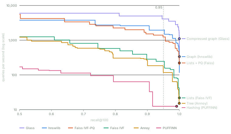— VIBE, 1.3 million arXiv abstracts in 768 dimensions, one core, recall@100. Each curve shows each implementation's best configuration at each recall level.

The table gives each family's values at a recall of at least $0.95$ , with the memory the index takes up and how long it takes to build, on one core. The original vectors take up 4.1 GB.

Family	Implementation	Queries per second	Index memory	Build
Hashing	PUFFINN	12	9.5 GB	35 min
Random trees	Annoy	117	12.0 GB	47 min
Inverted lists	Faiss IVF	246	5.7 GB	10 min
Lists with RaBitQ	RaBitQ IVF	983	0.7 GB	1.3 min
Lists with PQ and reranking	Faiss IVF-PQ	1,239	4.5 GB	1.4 min
Graph	hnswlib	2,001	4.5 GB	52 min
Compressed graph	Glass	4,125	2.8 GB	15 min

Three things stand out.

The order of the families. It's the same order the rest of the article follows, and the one VIBE reaches across its tests as a whole: graphs first; inverted lists with compression, close behind; trees and hashing, one or two orders of magnitude behind. The graph answers eight times more queries than uncompressed inverted lists, seventeen times more than the forest of trees and 160 times more than LSH. And compared with having no index: on ANN-Benchmarks' million 960-dimensional vectors, hnswlib answers 351 queries per second at recall 0.95, against brute force's 2.6, about 130 times more.

Compression isn't only for saving memory. Inverted lists go from 246 queries per second to more than a thousand when comparing with PQ codes instead of full vectors, and to almost a thousand with RaBitQ, in an index of 0.7 GB, less than a fifth of the original data. Faiss's IVF-PQ takes up more because it also keeps the full vectors for reranking. And the fastest index in the table, Glass, a graph library, walks the graph with vectors compressed to half a byte per number and reranks with half-precision vectors, two bytes per number.

The price of the graph is building it. hnswlib takes 52 minutes to build what Faiss's IVF-PQ builds in a minute and a half, about 38 times longer. For data that gets rebuilt often, that weighs as much as search speed.

Two caveats. VIBE measures one core and one query at a time; with batches of queries on a GPU the picture changes scale, and in the same benchmark CAGRA, NVIDIA's GPU graph, goes beyond 100,000 queries per second at recall 0.95. And these are vectors from a single model over a single kind of text. On VIBE's other datasets graphs stay on top, but when the queries don't look like the data, as when searching images with a sentence, even the best indexes get noticeably worse.

A dedicated vector database, or the one you already have?

The algorithms don't settle this question, because they're the same on both sides. pgvector offers HNSW and IVF; Oracle, HNSW and IVF; SQL Server 2025, DiskANN; Elasticsearch and MongoDB Atlas, HNSW. What changes is everything around them.

In favour of the database you already have, the vectors live next to the rest of the data: in the same transaction, with the same permissions and the same backups. A filter is a WHERE, and it can be joined with any other table. And there's no second system to keep in sync with the first, which is where errors tend to show up, when a vector and the data it came from stop matching.

In favour of a dedicated one: more indexes and more kinds of compression, on-disk indexes, filters inside the graph walk, sharding across machines when the data doesn't fit in one, and not paying for the rest of a SQL engine on every query. In ANN-Benchmarks, with the same data and recall 0.90, hnswlib answers 781 queries per second and pgvector, also with HNSW, 69; part of the difference is each query's trip through the connection and the SQL executor. There are concrete limits too: pgvector indexes vectors of up to 2,000 dimensions, or 4,000 in half precision, so the 3,072 of some current models don't fit in its index without reducing them.

A reasonable rule: if your data is already in PostgreSQL and the index fits comfortably in the server's memory without taking it away from the rest of the database, start with pgvector. A million 768-dimensional vectors with HNSW come to about 3.2 GB. When the index stops fitting, when queries per second are counted in thousands or when filtering demands more than asking for more candidates, a dedicated database starts to repay what it costs to run.

What to take away

If you take away one thing, let it be this: a vector index doesn't find the $k$ nearest. It almost always finds almost all of them, and the "almost" is a parameter you choose. In hundreds of dimensions, no exact index avoids ending up comparing almost everything, so they all give something up. Trees and hashing, memory; inverted lists, whatever sits on the other side of their borders; graphs, fast building and deletion; compression, the precision of each distance.

And if you take away three more, let them be practical.

Measure recall on your own data. Take a few hundred real queries, compute their exact neighbours by brute force (it's slow, but you only do it once) and compare them with what the index returns. Without that, you don't know whether a change of parameters or of model has cost you results.

Tune at query time, not at build time. ef_search in HNSW and probes in IVF trade speed for recall without rebuilding anything, and can be raised only for the queries that need it.

Choose by size, by change and by filters. As long as latency allows it, brute force is exact and there's nothing to maintain. If the index fits in memory, use an HNSW graph. If it doesn't, use compression with reranking or an on-disk index such as DiskANN. If the data changes all the time, look at how your engine deletes. And if you filter a lot, check how it filters before a query returns four results where you asked for ten.

The algorithms in this article are between ten and fifty years old and were born outside databases. What vector databases did was turn them into something that accepts changing data, filters and more data than memory. So when choosing one, the useful question isn't which algorithm it uses, because almost all of them use the same ones, but what it does with everything else.