Four labs that share no data, no architecture, no hardware and no opinion on much of anything published the same paragraph between 2020 and 2024. GPT-3 was trained with Adam, , and weight decay . OPT, with AdamW, , and . Llama 2, with AdamW, , and . DeepSeek-V3, with AdamW, , and . The update rule fits in four lines, it was published in 2017 as a fix to another from 2014, and the three numbers that go with it haven't moved in five years or across continents.
And then, in fourteen months, three cracks. Kimi K2, in July 2025, a trillion parameters trained without AdamW. GLM-5, in February 2026. DeepSeek-V4, in April 2026, with 1.6 trillion parameters: the same lab that sixteen months earlier had written everybody's paragraph. All three use Muon, an optimiser that in December 2024 was a blog post.
| model | year | optimiser | decay | ||
|---|---|---|---|---|---|
| GPT-3 | 2020 | Adam | 0.9 | 0.95 | 0.1 |
| OPT | 2022 | AdamW | 0.9 | 0.95 | 0.1 |
| Llama 2 | 2023 | AdamW | 0.9 | 0.95 | 0.1 |
| DeepSeek-V3 | 2024 | AdamW | 0.9 | 0.95 | 0.1 |
| Kimi K2 | 2025 | Muon | 0.1 | ||
| GLM-5 | 2026 | Muon | |||
| DeepSeek-V4 | 2026 | Muon |
GPT-3 calls it Adam and cites the AdamW paper for the decay: it's the same algorithm. And the three at the bottom haven't dropped AdamW entirely. DeepSeek-V4 keeps it for the embeddings, the output layer, the biases and the normalisations, and uses Muon for everything that is a matrix. That split isn't an implementation detail: it's the idea behind Muon, and this article ends on it.
It starts much earlier. Mathematical optimisation has spent two centuries accumulating methods, and a good share of them beat gradient descent on almost any criterion you care to measure: steps to arrive, sensitivity to the settings, guarantees. Newton's method, which is more than three centuries old, solves in a single step the problem gradient descent takes thousands on. Nobody trains with Newton. The question of this article is why, and the answer has three parts: why at this scale the only information you can pay for is the gradient, how each improvement to the descent buys back on credit something Newton had for free, and why the latest of those improvements is the one that has moved the throne.
The order is going to be logical, not chronological: each method fixes one specific failure of the previous one, and that order isn't the order of the dates. To have the dates in view:
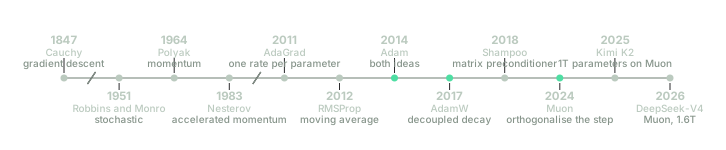
A hundred and sixty-four years between the first milestone and the fifth, and fifteen between the fifth and the last. The scale isn't uniform; the order is.
What there is to minimise, and what a step can cost
Let's call all the parameters of the model, stacked into a single vector with coordinates, and the loss: a number that measures how wrong the model is with those parameters, and which training means making small. For Llama 3 405B, is , and the loss is a mean over trillion tokens:
where is how wrong the model is on token and is those trillion. Three things about that definition decide everything that follows.
The first is that can't be evaluated. Computing it exactly means running the whole model over the tokens once, and that is, to a reasonable approximation, what the whole training run costs: a language model sees each token of the corpus once, or little more. Evaluating the exact loss a single time costs as much as training. Any method that asks for the exact value of at every step is ruled out before it starts.
The second is that the minimum isn't needed. isn't convex: it has many valleys, and no method you can run guarantees finding the deepest one. But that isn't what's being asked either. What gets measured is the loss of the model you ship, and a valley that isn't the deepest will do if it's deep enough. That concession is what makes everything else possible.
The third is the price of each kind of information, and it's worth putting numbers on it. Evaluating on a batch of data is one forward pass. Computing its gradient, the vector of partial derivatives that says which way the floor is from here, costs roughly two more forwards, by the chain rule run backwards: three forwards in total, and a vector of numbers that takes as much room as the model. Computing the matrix of second derivatives, the Hessian , which says how much the loss curves in each direction, produces numbers. For Llama 3 that is . The H100 GPUs used to train it add up to bytes of memory, and storing that Hessian in the lowest precision anyone trains in asks for million times that. You don't even need the whole matrix for it to go wrong: the product of with a single vector, which gives the curvature in one direction only, costs about as much as an entire gradient.
That is the asymmetry everything comes from. With one gradient you know which way is down in all directions at once, and it costs three forwards. Knowing how much the loss curves in one direction costs the same, and knowing it in all of them fits nowhere.
The catalogue, ordered by what each method asks for
Mathematical optimisation methods can be sorted into four families by the kind of information they demand about the loss in exchange for a step: values of the function only, a promise about its shape, its second derivatives, or its first derivatives only. That is the order this section follows, and it leaves for last the family training actually uses.
Derivative-free. Grid search, random search, the Nelder-Mead simplex of 1965, genetic algorithms, evolution strategies, Bayesian optimisation. They all ask for the same thing, which is the minimum: evaluate at points of their choosing. They differentiate nothing, and in exchange they have to work out where the floor is by comparing values, and in dimensions there are independent directions to compare. Approximating the gradient by finite differences costs evaluations, against the three it costs to compute it. Evolution strategies estimate it more cheaply, perturbing the parameters at random and keeping the perturbations that lower the loss, and in 2017 they taught a simulated humanoid to walk in ten minutes by spreading the work over more than a thousand processors. But the noise of that estimate grows with , and has grown a hundred thousand times since. What you save by not differentiating you pay times over in evaluating.
Structured. Dantzig's simplex of 1947 and the interior-point methods solve linear programs with hundreds of thousands of variables; quadratic programming and the whole of convex optimisation, with its subgradients, its proximal methods and its guarantees that the minimum found is the only one, solve enormous problems in seconds. What they ask in return isn't information about but a promise about its shape: that it be linear, quadratic or convex. A network's loss is none of the three, and there is no way to make it believe otherwise.
Second order. Here is the method that solves the problem, and it's worth seeing why. Near the loss looks like its second-order approximation, a quadratic with the gradient as the linear term and the Hessian as the curvature:
If that approximation were exact, the best step would be the one that minimises it. Differentiating with respect to and setting to zero gives , that is,
which is Newton's method. It has no learning rate: the size of the step is decided by the curvature, and decided separately in each direction. Where the loss curves a lot the step is short, and where it curves little the step is long, without anyone having to say so. Newton has for free what everything else is going to have to pay for: the curvature of every direction.
What it costs has already been said: numbers to store , and on the order of operations to solve the system. The quasi-Newton methods were born to avoid paying that. BFGS, named after its authors Broyden, Fletcher, Goldfarb and Shanno, is one of the best known. Instead of computing the Hessian it builds an approximation to out of how the gradient changes from one step to the next, which is information you already have. It still takes . L-BFGS (limited-memory BFGS), proposed later, avoids storing the whole approximation to the inverse Hessian: it keeps only the last pairs of changes, with between five and twenty, and from those it rebuilds the product in operations and of memory. That you can pay, and for twenty years it was machine learning's default: logistic regression, conditional random fields, support vector machines with a linear kernel. In 2011 it was tried on deep networks, and on some problems it held its own against gradient descent.
It fell over two things it needs that a batch of data can't give it. The first: the pair of changes it uses to update its approximation, how far moved and how much the gradient changed, only makes sense if both gradients were computed on the same data; with different batches, the difference between the gradients is mostly the difference between the batches, and that difference goes into the estimate of as if it were curvature. The second: to decide how far to go in the direction it proposes, L-BFGS runs a line search, which tries several step sizes and keeps one that lowers the loss enough, and to know whether the loss has gone down you have to be able to evaluate it. Both ask for exact values, and the first section said what one of those costs. The Hessian-free methods of 2010 tried the other route: don't store , use only products, each at the price of a gradient, to solve Newton's system by conjugate gradient. It came to tens or hundreds of products per step. In that time, gradient descent takes tens or hundreds of steps.
First order. What's left. One gradient per step, three forwards, numbers of memory, and no promise about the shape of .
| family | asks per step | cost per step | memory | tolerates a noisy gradient? |
|---|---|---|---|---|
| derivative-free | evaluations of | forwards | yes | |
| structured | that be linear, quadratic or convex | depends | depends | not applicable |
| Newton | gradient, Hessian and solving a system | no | ||
| L-BFGS | one gradient and pairs of changes | no: secant and line search | ||
| first order | one gradient | forwards | yes |
The last column is the one that decides, and it deserves its own paragraph, because the reason gradient descent doesn't only survive but suffices is there and not in the cost. The loss is a mean of terms, so its gradient is the mean of gradients, and the mean of a handful of them chosen at random is an unbiased estimator of the mean of all of them: it points, on average, at exactly the same place, and it costs whatever the handful costs. The Hessian can be estimated that way too. What can't be estimated that way is its inverse, which is what Newton needs: the inverse of a noisy estimate isn't an estimate of the inverse, and the noise in the gently curved directions, which are the ones with small entries in , comes out amplified by the inversion. The gradient is the one piece of information that is both cheap and estimable without bias from a slice of the data.
Everything from here on can be read this way: gradient descent is the only thing you can pay for, and each of its improvements is a way of approximating that survives the noise. The diagonal, in RMSProp and Adam. A product of small matrices, in Shampoo. The spectrum of each weight matrix, in Muon. Each buys back a piece of what Newton had for free, at a price you can pay.
Gradient descent, and the one number you choose
In 1847, Cauchy presented to the Paris Academy of Sciences a three-page note for solving, without isolating anything, the systems of equations that give the orbit of a heavenly body. The idea fits in a sentence: wherever you are, look at which way the function climbs fastest and move a little the opposite way. What takes an article is what "a little" means.
The gradient collects one partial derivative per parameter: each coordinate says how fast the loss changes when that parameter moves and the others stay put. That it's the direction of fastest ascent isn't a definition but a theorem, and it comes out of an inequality. Take any direction of length ; how much the loss changes when you move a little along it is the directional derivative, which is a dot product, , and by Cauchy-Schwarz that product is bounded by , with equality only when is parallel to the gradient. No direction climbs more per unit of step than the gradient's, so none descends more than the opposite one. From there, the whole rule:
where counts steps and is the learning rate, the one number in the formula that you choose. That every step lowers the loss can be seen with the tangent plane:
and with the loss drops by , which isn't negative. The whole debt is in the : it holds near , and how near is decided by .
The arithmetic comes out whole on a parabola
Take the smallest loss there is, a single parameter and , with derivative . The rule becomes : multiply by the same constant at every step. Iterating from ,
and a power tends to zero if and only if its base measures less than . The condition is , that is , and the factor itself tells you what happens in each range: between and the weight shrinks without changing sign; at it lands on the minimum in a single step; between and it alternates sign and shrinks; at it alternates forever; above that, it alternates and grows.
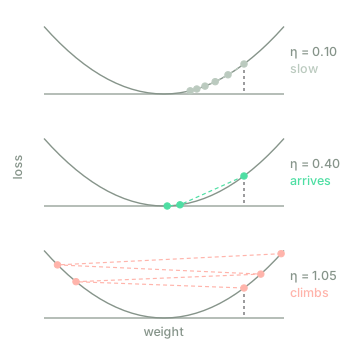
The two failures are opposites: the short step always goes down and never quite arrives, and the long step crosses the bottom and comes out higher than it went in. There is no step size that's right by nature; there is one that depends on how much the loss curves.
That in the limit belongs to this parabola. With the derivative is , the factor becomes and the condition becomes : the more the loss curves, the shorter the step has to be. So far nothing hurts, because is one number and is chosen by looking at it.
One rate for two curvatures
It hurts as soon as there are two directions that curve differently, and a network has . The function is the least you need to see it: an elongated ravine, nearly flat along and very steep along . The parabola's arithmetic, coordinate by coordinate, asks for for and for , and the second one rules. The per-step factors are in and in .
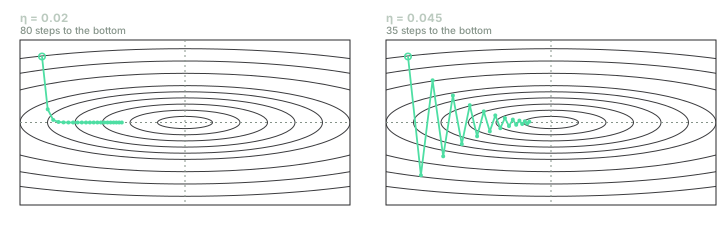
The same ravine, the same starting point. With the factors are and : the steep coordinate reaches the bottom in three steps and the flat one advances 4% per step, and takes . With they are and : the flat one goes twice as fast, and the steep one crosses the bottom at every step and bounces off the opposite wall. It arrives in , zigzagging.
The two trajectories are the same dilemma seen from each side. A small rate respects the steep direction and wastes the flat one; a large one exploits the flat direction and bounces in the steep one. No serves both well, because is one number and the curvatures are two.
The ratio between the largest curvature and the smallest is called the condition number, , and here it's . Let's call the curvature in the steepest direction and the curvature in the flattest. The condition number rules the number of steps: the best possible is on the order of , and with it the flat direction contracts by a factor per step, so reaching a given precision costs a number of steps proportional to . In a network, computing that can't be paid for, but there is a measurement that repeats in every model anyone has looked at: the most and least curved directions differ by several orders of magnitude. In a ravine with we're talking a few tens of steps. One a hundred times narrower, in the Adam section, is going to cost .
The problem has a name, ill-conditioning, and everything after this section is a way of treating it. Newton treats it by dividing by , and that can't be paid for. The rest are ways of approximating that division with what can.
Stochastic: the gradient nobody can compute in full
Before treating the ravine there's the other problem from the first section to deal with, and it comes first: the exact gradient costs as much as the whole training run, so nobody computes it. What gets computed is the gradient over a batch of examples chosen at random,
and that is what gets subtracted. It's an estimator: its mean over all possible batches is exactly , because the gradient of a mean is the mean of the gradients, and its variance shrinks like . It costs what costs, not what costs. For Kimi K2, each batch is million tokens out of a corpus of trillion: each step looks at % of the data and points, on average, at the same place it would if it looked at all of it. For the compute of a single exact step you get two hundred thousand noisy ones, and the noise averages out along the way.
That is stochastic gradient descent, SGD, and it isn't an approximation to the method but a theorem from 1951 about how to find the zero of a function you can only observe with noise. Robbins and Monro proved that the iteration converges if the rate decreases in a specific way: the sum of all the has to diverge, so the method can travel any distance, and the sum of their squares has to converge, so the noise eventually dies away.
The noise Robbins and Monro talk about is, in our case, the difference between the gradient we compute and the one we would like to compute: the batch's minus the exact one,
It has mean zero, on average we point at the right place, but it isn't free. It costs three things, and all three matter later. The first is that an individual step can raise the loss; the descent guarantee of the previous section becomes a guarantee on average. The second is that near the bottom the trajectory doesn't stop: it trembles with an amplitude proportional to times the size of the noise, and the only way to settle it is to lower . That is why no model trains at a constant rate to the end. The third is the one that closed the door in the previous section: with a noisy gradient, the line search can't tell whether the loss went down and the secant condition measures noise. The second-order methods didn't lose on cost alone; they lost because the noise contaminates the curvature estimate, and the convergence guarantees that survive that noise are the first-order ones.
There is one thing the noise gives you, and it's worth saying carefully because it has been exaggerated a lot. A saddle point, where the gradient is zero but the loss goes down in some direction, is an unstable equilibrium: exact descent stays parked on top of it, and the noisy kind needs only a nudge in any downhill direction to leave. In high dimension, almost all the points where the gradient vanishes are saddles and not minima, so this isn't a detail. But it isn't what makes SGD work; it's what keeps it from getting stuck.
With that, the method that trains every model in the table is complete: a noisy gradient, subtracted with a decreasing rate. What's missing is making it bearable in a ravine, and that is where the variants start.
Momentum: remembering the previous step
The ravine's zigzag has a property you can exploit: in the steep direction the gradient changes sign at every step, and in the flat one it keeps it. A method that averages recent gradients cancels the first and accumulates the second, without knowing which direction is which. Polyak proposed it in 1964 with a physical image, a heavy ball rolling over the surface and keeping part of its velocity, hence the name:
with between and , and nearly always . To keep things short, we write . Unrolling the first line, is a sum of all the previous gradients with geometrically decaying weights:
With that, the arithmetic of the two directions comes out whole. If the gradient is always the same, , the sum tends to : with , ten times the gradient, and the effective step is ten times . If it alternates between and , the sum tends to : little more than half. The same rule amplifies tenfold the direction the gradient insists on and halves the one where it contradicts itself. Averaging in time tells apart what the learning rate couldn't.
What doesn't change is that there is still a single . Momentum doesn't remove the steep direction's limit, it moves it: with the parameters well chosen, the number of steps to a given precision goes from proportional to to proportional to , and the well-chosen parameters depend on , which nobody knows.
Nesterov proposed in 1983 a variant that evaluates the gradient not where the ball is but where it's going to be after the push, a step of anticipation that improves the theoretical guarantee, and in 2013 it was shown to train deep networks better. The difference from Polyak's is small in practice; it matters in the last section, because Muon uses Nesterov's.
One rate per parameter: AdaGrad and RMSProp
The other attack on the ravine doesn't average in time, it rescales in space: instead of one , one per parameter, and let the method itself choose them. The rule is to divide each coordinate of the gradient by a measure of how large that coordinate's gradients have been. AdaGrad, from 2011, accumulates their squares:
where the square, the root and the division are coordinate by coordinate, and is a tiny number that avoids dividing by zero. It was born for problems with rare inputs. Think of a language model: the embedding row of a word only receives gradient at the steps where the word appears, and most words appear rarely. With a shared , the frequent words set the limit and the rare ones barely move. With AdaGrad, each parameter has its own : those that receive gradient at every step accumulate it fast and slow down, and those that receive it once every thousand steps keep taking large steps. This comes back later, because it's a good part of the reason a language model isn't trained with plain SGD but with methods that adapt the rate parameter by parameter.
The flaw is in plain sight: only grows, so the effective rate only falls, and on a non-convex problem, where you have to keep moving after a long time, it ends up stopping before it arrives. RMSProp fixes that by swapping the sum for an exponential moving average, which forgets:
That average's memory is about steps: ten with , a thousand with . RMSProp was never published. It's a slide from a 2012 online course of Hinton's, and for years it was cited that way, "Lecture 6.5", because there was nothing else to cite.
What it does on the ravine, , can be seen without drawing it. In the steep direction the gradient is ; in the flat one, . Dividing each by the root of its own mean of squares, which is more or less its magnitude, leaves in each coordinate a step of size with the gradient's sign, whatever its scale: the step has stopped depending on the curvature. That is exactly a diagonal approximation of with the gradient magnitudes standing in for the curvature, and it costs one more vector of memory. Second order comes back in through the window, as a diagonal, at a price you can pay.
It has a start-up defect worth measuring, because it's the one Adam is going to correct. At the first step , so the division leaves per coordinate: with that is , and with it is . On the ravine, with and , the first step takes the trajectory from to : it crosses the bottom and comes out the opposite wall, because the moving average hasn't seen anything yet and underestimates the size of the gradient thirty times over.
Adam: both ideas together
Adam, from December 2014, joins the two: a moving average of the gradient, which is momentum written as an average, and a moving average of its square, which is RMSProp.
And it corrects the start. Unrolling as before, it's times the sum of the gradients with weights ; if all the gradients were equal to , the geometric sum gives . At the first step the average is , a tenth of the gradient; at step , a fraction that climbs towards . Dividing by that fraction restores the correct scale from the first step, and the same for with :
With that correction the first step is per coordinate, with the gradient's sign, and not . Those are the four lines from the table at the top, and two more vectors of memory, and , the size of the model.
The reading that explains why it works on almost everything is in the quotient. estimates the mean of the gradient and estimates the root of the mean of its square, and the first never exceeds the second in absolute value. The quotient lies, coordinate by coordinate, between and : near where the gradient insists on a sign, near where its mean is noise. No parameter moves more than per step, whatever the scale of its gradient. That is why can be chosen in units of the parameter, why the same works for models that have nothing in common, and why a rate of means something concrete: no weight changes by more than three ten-thousandths per step.
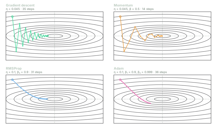
The four methods on the same ravine, from the same point, twenty steps drawn and the total to the bottom in each label. Momentum carries rather than the usual because the is meant for ravines some seventy times narrower than this one, and here it overshoots in the flat direction. RMSProp and Adam take steps of the same length in both coordinates: the -degree diagonal is the signature of the rescaling.
Look at the steps to the bottom before drawing conclusions: Adam takes and the descent . On a ravine with and a well-chosen rate, Adam isn't faster. Its advantage is something else, and to see it you have to change the ravine without changing the rate.
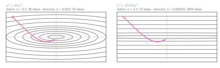
On the right, the same ravine a hundred times narrower. Gradient descent needs a rate a hundred times smaller to avoid diverging, and with it takes steps. Adam takes the same thirty steps as on the left, with the same , and arrives in . Nothing had to be touched.
That is what Adam buys: not speed on a known problem, but independence from the curvature on an unknown one. A network has millions of ravines of different widths inside it, and nobody is going to measure any of them.
The W: a regularisation mistake that lasted three years
Almost every model is trained with weight decay: at every step, besides subtracting the gradient, each weight gets shrunk a little towards zero, , so that none of them grows without bound. Under gradient descent that is identical to adding a term to the loss, the L2 regularisation, because the gradient of that term is and subtracting it with gives the same formula. Two names, one algorithm, and for decades nobody had to tell them apart.
Under Adam they stop being the same thing, and the arithmetic shows it. If the decay enters as a term of the loss, it enters , and from there and : it goes through the division. For a parameter with historically large gradients, is large and its comes out divided by a large number: it barely decays. For one with small gradients, it decays in full. The strength of the regularisation comes to depend on each weight's gradient history, and in the opposite direction to the sensible one: the weights that move the most are the ones held back the least.
Loshchilov and Hutter pointed it out in November 2017 and proposed taking the decay out of the division:
That is AdamW, and the W is weight decay, decoupled. The difference from the previous formula is where sits: outside the quotient, instead of inside . At the time there was a result from that same year according to which Adam generalised worse than SGD with momentum in vision, and a good part of that gap was this: Adam was regularising itself badly. With the decoupled decay the distance closed on the tasks they tried. The in the table at the top is the of this formula, and it gets multiplied by : with , each weight shrinks by three hundred-thousandths per step.
Why AdamW, and why with those numbers
So far, the generic answer: Adam joins the two ideas and AdamW fixes its regularisation. The concrete question is why a transformer isn't trained with SGD with momentum, which worked in vision for years and keeps a single state vector instead of two, and the answer has been slow to arrive.
It's in the rare words, which are almost all of them. A language model's loss is a mean over tokens, and tokens follow Zipf's law: a few appear in every batch and the vast majority once every many thousands. The parameters that touch only a rare token, its row in the embedding matrix and its row in the output layer, receive minuscule gradients on average, and under SGD a minuscule gradient is a minuscule step. Those parameters don't learn, and the loss on the rare tokens, which are most of the vocabulary, doesn't go down. Kunstner and others measured it in 2024 class by class, and it is AdaGrad's problem as is: one rate per parameter is what lets a rare word's row advance as much per step as a frequent one's. On top of that, the gradient noise in a model with attention has heavy tails, occasional batches with enormous gradients, and the scale of the gradients differs by orders of magnitude between the embeddings, the attention matrices and the normalisations. They're ravines inside ravines, and SGD has one for all of them.
The numbers in the table each answer to a failure with a name.
and not the original paper's . The memory of is steps: a thousand with , twenty with . With a thousand steps of memory, when a batch suddenly brings a large gradient in some coordinate, takes hundreds of steps to find out, and meanwhile is far above in that coordinate: an enormous step, and the loss jumps. Those are the loss spikes that keep everyone who trains at this scale awake. With twenty steps of memory, reacts sooner. GPT-3 set and nobody has had a reason to go back.
Gradient clipping to norm . Before enters and , if its norm exceeds it gets rescaled to . It's the other defence against the heavy tails: an atypical batch can't push the averages around.
. In the original paper it's ; Llama 2 used , and OLMo 2 went back to because with the parameters whose gradients are smaller than that, which in a large model are many, see their step held back by the instead of by . A number that exists to avoid a division by zero ends up deciding how much the quietest parameters learn.
Warmup. The bias correction fixes the mean of in the first steps, not its variance: estimated from three or four gradients, is so noisy that the quotient can take large steps in wrong directions. The RAdam analysis showed that raising the rate linearly from zero over the first few thousand steps is exactly a cure for that. Llama 2 warms up for steps; Llama 3, for .
Schedule. After the warmup, cosine down to % of the peak rate in GPT-3 and Llama, or a long constant stretch followed by a cooldown in DeepSeek-V3 and Kimi K2, which hold the rate fixed for the first ten trillion tokens and only then bring it down. The two shapes give equivalent results, and both are Robbins and Monro's second condition made cheap: sit at the highest rate the training run can stand for most of the time, and lower it at the end to settle the trembling.
Then there's the bill. and are two vectors the size of the model, and for billion parameters in single precision they take TB: forty GB H100s dedicated to remembering. That bill is where the last section starts.
What comes next: per matrix, not per coordinate
Adam costs two things, memory and a diagonal approximation, and what has been proposed since attacks one of the two.
Less memory. Adafactor, from 2018, doesn't store the whole for an weight matrix: it stores the row sums and the column sums, numbers instead of , and rebuilds the matrix as their product. T5 was trained that way. 8-bit Adam stores and quantised. Lion, from 2023, found by automatic search over programs, keeps only momentum and uses as its step the sign of a blend of the momentum and the gradient: one state vector instead of two, and the sign is the extreme case of Adam's rescaling, where every step measures exactly .
More curvature. Here is what has changed the table. Adam treats the numbers of a weight matrix as parameters with no relation to each other, and they aren't: the matrix multiplies a vector, and its gradient is a matrix too, with rows and columns that mean something. Shampoo, also from 2018, preconditions with two small matrices instead of a diagonal, one on each side:
is and is : for a square matrix, twice Adam's memory and not its square, and in exchange an approximation of that is no longer diagonal. It took six years to make it run at scale, and in 2024 it won the AlgoPerf competition training % faster than the reference, an AdamW with Nesterov momentum. SOAP puts Adam inside the basis Shampoo computes.
Muon does something more radical with the same premise. Instead of preconditioning the gradient, it takes the momentum matrix of each weight matrix and replaces it with the nearest orthogonal matrix: if is its singular value decomposition, the step is
the same matrix with all its singular values set to . Computing that decomposition would be expensive; the December 2024 blog post that proposed it approximates it with five iterations of a polynomial in , matrix products only, in low precision. Compare with what came before: Lion normalises each number, Adam normalises each coordinate by its recent magnitude, and Muon normalises each matrix by its spectrum. It's the same rescaling one level up. And the argument for why it helps is the ravine once more, inside each matrix: the gradient of a transformer layer is nearly low-rank, a few directions dominate it, and orthogonalising it gives the rare directions the same step size as the dominant ones. There is a reading that puts all three in the same formula: each is steepest descent under a different norm, and choosing the optimiser is choosing what "a step of size " means.
Muon exists only for matrices. The embeddings, the output layer, the biases and the normalisation weights stay on AdamW in every model that uses it, and that is why the last three rows of the table are, strictly, Muon and AdamW at once. What took Muon from an experiment to a production model were two additions from February 2025: weight decay, and a rescaling of the step so that AdamW's and carry over without a new search. With that, Moonshot trained a -billion-parameter model on trillion tokens and reported twice AdamW's compute efficiency. Five months later, Kimi K2: a trillion parameters, trillion tokens and, by its own report, not a single loss spike. Then GLM-5 and DeepSeek-V4, which justifies it in two words, convergence and stability.
No schedule. The other line doesn't touch the direction of the step but the rest of the recipe. Schedule-Free AdamW replaces the rate schedule with an average of the points the trajectory passes through, and it won the no-hyperparameter-tuning track of the same AlgoPerf. It's the only one of these proposals that removes a number instead of adding an idea.
It's worth ending with the fair measurement. The most careful comparison to date, eleven optimisers each with its learning rate tuned, from to billion parameters, found that the announced gains, of to times, came partly from comparing against a badly tuned AdamW; that the real gains exist and all belong to the methods that precondition per matrix, Muon, SOAP and their relatives; and that they're worth times on the smallest model and on the largest, shrinking as the model grows. % of the compute of a frontier training run is still a lot of money, and the stability DeepSeek cites isn't measured in that table. But the picture is more modest than the announcements and firmer than the scepticism: the gains belong to the matrices, and they're the ones that last.
What to take away
If you take away one thing, let it be this: the optimiser of language models wasn't chosen for being good, it was chosen for being affordable. Newton had the curvature of every direction and solved it in one step; at this scale it fits nowhere and doesn't survive the noise. Everything that has happened since Cauchy is buying back on credit what Newton had for free: momentum averaging in time, RMSProp rescaling per coordinate, Adam with both, AdamW fixing what the rescaling had broken, and Muon rescaling per matrix. The gradient descent rule hasn't changed by a letter. What changes, each time, is what a step can cost.
And if you take away three more, let them be practical.
The defaults aren't arbitrary, and knowing what each answers to tells you when to touch it. is against the spikes; clipping to , against atypical batches; the warmup, against the variance of at the start; the rate decay, Robbins and Monro's condition; the of weight decay, the regularisation that Adam without the W applied backwards. If you're training something small and calm, the original for is reasonable; if you see spikes, you know which number to look at first.
The learning rate is still the number. In Adam it comes in units of the parameter, so means no weight moves more than that per step, and that meaning doesn't depend on the model. Before trying another optimiser, sweep : a good part of the gains announced in recent years were explained by an AdamW whose rate nobody had swept.
If you're fine-tuning a model that isn't yours, the optimiser's memory decides whether it fits. and take twice the room of the weights, and every answer you've seen to that, LoRA, 8-bit Adam, Adafactor, is a way of not paying the bill from the Adam section. And if what you train is matrices, Muon for the matrices and AdamW for the rest is, today, what three of the largest models ever published do.
Back to the table. Four labs wrote the same paragraph because they arrived at the same price. Three have rewritten it because they found how to pay a little more of what Newton had for free: not the curvature of each coordinate, but that of each matrix. Gradient descent is still subtracting the gradient. What has changed, once again, is what fits in a step.