"El niño juega en el jardín." Six Spanish words and a full stop. The tokeniser that GPT-2 was trained with in 2019 needed twelve tokens to write it down, and its English translation, "The boy plays in the garden.", got by on seven. In 2022, with the tokeniser GPT-3.5 and GPT-4 use, Spanish came down to eleven. In 2024, with GPT-4o's, it came down to seven: exactly as many as English, and this time with the words whole.
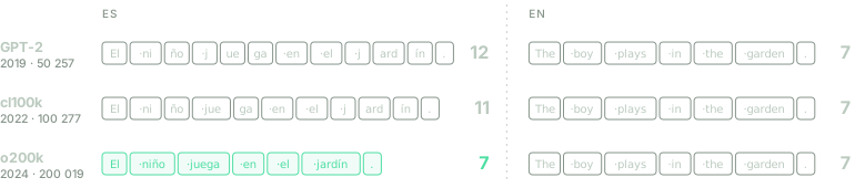
The same sentence and its translation, cut by three generations of the same tokeniser. The dot inside a box marks the space that token carries glued to its front. English does not move: seven tokens and the same seven pieces all three times.
English stood still. Seven tokens across the three generations, and cut in the same places all three times. What moved was Spanish, and not because anyone fixed it: the language does not enter into the equation. What changed was the size of a list, and who was on it.
This article is about how that list gets built. I go through it in the order it happened, because that order is what makes it make sense: how text was cut before any of this existed and why that way of cutting stopped working, where BPE came from (a compression algorithm from 1994 that was given a different job), what really separates the three methods in use today, why a floor made of bytes ended up underneath all of them, and what the choice still costs you when the text you write is not English.
Not one of those decisions was taken with Spanish in mind.
The age of the word, and why it ended
A language model does not read text, it reads numbers. Before any network gets involved, someone has to break the string of characters into units and give each unit an index. Those units are called tokens, the closed list of the ones the model recognises is the vocabulary, and the program that decides where to cut is the tokeniser.
The index on its own says nothing: "casa" being entry 412 and "perro" entry 413 does not make them alike, any more than two consecutive phone numbers belong to two neighbours. What the model learns is a vector of numbers for every vocabulary entry, its embedding, with the same for all of them: a few hundred in small models, a few thousand in large ones. Stacked, those vectors form a matrix of that is trained along with the rest of the network, and at the end of the model there is another matrix of the same size in the layer that decides which token comes next.
That is why the vocabulary is fixed before training and never touched again: every entry costs two rows of numbers, and the number of rows has to be known before you start. It is finite, closed and expensive. Language is none of the three, and everything that follows comes out of that collision.
For decades, deciding where to cut meant writing rules. A tokeniser of that era was a list of cases: cut on spaces, separate the final punctuation from the word but not the full stops in "EE. UU.", keep opening and closing quotes together, decide what to do about hyphens. The two most used in research, Penn Treebank's and Moses', were exactly that, and they came with the small print: the rules are per language. The one that knows "don't" is two words knows nothing about "dámelo", and neither is any use for Chinese, which does not separate words with spaces.
The underlying problem was not the rules, which can be written. It was the size of the list they produced.
To see it in numbers rather than adjectives, I put together three public-domain Spanish books, all from Project Gutenberg and all downloadable as plain text: Don Quijote, by Cervantes; La Regenta, by Leopoldo Alas; and Amar es vencer, by Pauline Caro. That is 746,368 words in total, counting as a word any sequence of symbols separated by a space and lowercasing everything.
The vocabulary that comes out has 38,792 distinct words, and it is distributed the way it always is in any language: a word's frequency is inversely proportional to its rank,
with an that is in this corpus. Ten words ("de", "que", "y", "la", "a"…) take an enormous share of the text, and behind them comes a tail that never ends. Quantify it: of those 38,792 distinct words, 17,536 appear exactly once. Nearly half the vocabulary exists to be used a single time in 746,368 words.
That is already uncomfortable, because every vocabulary entry costs one row of numbers to represent it and another in the output layer, so there you are paying two rows for one appearance. But the serious part is the other one: the list never stops growing. Having read half the corpus you had seen 22,643 distinct words; reading the other half brings 16,149 more. The text doubles and the vocabulary grows by 71%.
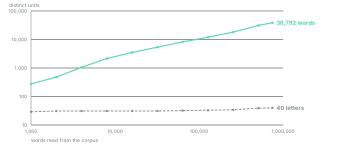
The same 746,368 words counted two ways, on logarithmic axes. As a vocabulary of words, the count climbs without bending anywhere. As an alphabet, it settles inside the first thousand words and stops moving: the eleven letters that turn up later are rare accents and characters from other languages.
That curve has a name and a closed form. It is known as Heaps' law, and it says the vocabulary grows as a power of the text read:
Here is how many words you have read (746,368 at the end of the corpus), how many distinct ones have appeared by that point, and and are two constants fitted to the corpus: sets the height of the curve and , the one that matters, its slope on the logarithmic axes of the figure. In any language falls between and ; in this corpus it is , with . That is less than means each new word is a little harder to find than the last; that it is greater than means you will never stop finding them. There is no corpus size beyond which the vocabulary is complete, and there is none because Spanish is not a list: it is a machine for generating words, with its conjugation, its diminutives and its knack for gluing two clitics onto an imperative.
What the first generation of neural machine translation systems did was the only thing they could do: cut the list wherever it could be afforded. The cut was not aesthetic, it was arithmetic. The layer that decides the next word computes a score for every vocabulary entry, which costs on the order of operations at every step of every sentence, with the same as the embeddings. With in the hundreds of thousands, that layer alone eats the budget. Hence the vocabularies of 30,000 to 80,000 words in those systems, and hence there being work devoted purely to being able to use a larger vocabulary.
And the words left outside? They were replaced by a single symbol, UNK, and on you went. Measure
what that means on the corpus above: train the vocabulary on 90% of the text and read the remaining
10%. 4.8% of the words you read are not in the vocabulary, and they are not oddities, it is one
in every twenty ordinary words. All of them reach the model as the same symbol, indistinguishable
from one another: the proper noun, the technical term and the typo share a representation. And since
translation has to produce text, UNK came out the other side as well, so people had to
invent patches that noted where each UNK came from in order to
copy the original word or look it up in a dictionary afterwards.
A tokeniser that needs a patching system for the words it could not represent is saying, under its breath, that the chosen unit is the wrong one.
The flight to the character, and what it costs
If the problem is that words run out before the language does, there is an obvious way out: do not use words. Use letters. The vocabulary becomes the alphabet, a few dozen symbols, and in the figure above it is the flat line: with a thousand words read you have already seen almost every letter Spanish uses, and reading a million more adds practically none.
Everything that hurt is fixed at a stroke. No UNK is possible, because any word that arrives is
written with letters already in the vocabulary. The output layer stops being the bottleneck, because
deciding between forty symbols is free compared with deciding between fifty thousand. And related
words stop being strangers to each other: "niño" and "niña" share three of their four letters,
something a vocabulary of words cannot even state. There were serious character-level models, and
they worked.
The price shows up the moment you count the steps. Call the number of characters in a text, the number of tokens a tokeniser breaks it into and the mean length of those tokens, in characters. Tokens are pieces of the text itself, so their lengths add up to the whole text and the three quantities are tied together:
The text fixes , so and do not move independently: the shorter the pieces, the longer the sequence, and there is no way to have both. Cutting by characters, and therefore . On the corpus above that means where the word tokeniser saw 746,368 units, the character one sees 4,194,315: nearly six times as many steps for the same text.
And the cost is not multiplied by six but by rather more, because the parts that compare each position with all the others (attention, which is what today's models are made of) grow as :
Thirty-two times the work, for the same text and to learn how to spell along the way. There is a second cost, less visible and worse: the distance between two related words in a sentence is multiplied by six too, so the model has to hold much longer dependencies to discover the same thing.
With the two obvious ways out ruled out, the trade-off is visible whole:
| cut | |||
|---|---|---|---|
| characters | dozens, and it saturates | ||
| subwords | – | 30,000–200,000, chosen in advance | |
| words | tens of thousands, and growing |
The middle row is the one that won, and its right-hand cell says what it consists of: instead of letting the size of the vocabulary be a consequence of how you cut, it is fixed up front and an algorithm is left to decide which pieces make it up. Frequent words will end up as a whole piece and rare ones will be written with several, without anyone having to decide which are which.
So the flight to the character worked, and nobody stayed to live there. The answer turned out to be that nobody should choose the unit.
BPE: a compression algorithm repurposed
The algorithm that ended up solving this is called byte-pair encoding, BPE from here on, and the name says exactly what it does: encode pairs of bytes. It was published in 1994 in a magazine for C programmers, and what it wanted was to compress files. Find the most repeated pair of bytes, replace it throughout the file with a byte that does not appear in it, and repeat. Every one of those substitutions has to be written down so it can be undone later, and where they are written down is the substitution table: a list of lines saying "the byte 0xFE means the pair AB".
Twenty-two years later, a paper on machine translation took that algorithm out of compression and set it to do something else. They did not change the algorithm. They changed when it stops.
The difference lies in what you do with that table. When compressing it is a necessary evil that travels with the file, because without it nobody can recover the original. When tokenising, nothing is recovered: you stop at 30,000 substitutions because that is the vocabulary you wanted, and the table is the tokeniser. Everything a BPE tokeniser knows fits in that ordered list of pairs.
Training
The corpus is first counted by words, with their frequencies, and each word is split into characters
(characters, yes, despite the name of the algorithm; the actual bytes come back later, and not by
accident). An end marker, </w>, is glued to the end of each word, which stops a piece from crossing
from one word into the next and, above all, writes down where a space used to be. That second part is
a requirement, not a flourish: concatenating the tokens has to give back the text you started with,
spaces included, because a tokeniser that loses information along the way is no longer dividing the
text, it is altering it, and what the model is denied it will never see.
Let be the frequency of the word in the corpus and the number of times the pieces and appear adjacent inside . Summing over all words, and weighting each by how often it occurs, gives how many times that pair appears in the whole corpus:
On each round the pair with the highest count is merged,
and this is repeated as many times as you want pieces added to the vocabulary. That is all of it. There is no grammar, no morphology and no notion of a word beyond the end marker.
from collections import Counter

CORPUS = """
el niño juega en el jardín la niña juega en el jardín
el niño aprende programación la niña aprende programación
la programación se aprende programando y programando se aprende
el profesor enseña programación la profesora enseña programación
enseñar no es lo mismo que aprender el niño enseña a la niña
la niña enseña al niño programación y el niño aprende
"""

def pairs(vocab):
    """Count every adjacent pair of pieces, weighted by the word's frequency."""
    counts = Counter()
    for pieces, f in vocab.items():
        for pair in zip(pieces, pieces[1:]):
            counts[pair] += f
    return counts

def merge(vocab, pair):
    """Replace every occurrence of `pair` with the piece that results from gluing it."""
    a, b = pair
    updated = {}
    for pieces, f in vocab.items():
        out, i = [], 0
        while i < len(pieces):
            if i < len(pieces) - 1 and pieces[i] == a and pieces[i + 1] == b:
                out.append(a + b)
                i += 2
            else:
                out.append(pieces[i])
                i += 1
        updated[tuple(out)] = f
    return updated

def train(corpus, n_merges):
    # Every word starts split into characters. `</w>` marks where it ends.
    vocab = {tuple(w) + ("</w>",): f for w, f in Counter(corpus.split()).items()}
    merges = []
    for _ in range(n_merges):
        counts = pairs(vocab)
        if not counts:
            break
        pair = max(counts.items(), key=lambda kv: kv[1])[0]   # tie: the first one seen wins
        merges.append((pair, counts[pair]))
        vocab = merge(vocab, pair)
    return merges

for i, (pair, n) in enumerate(train(CORPUS, 15), 1):
    print(f"{i:2}. {pair[0]!r} + {pair[1]!r} -> {(pair[0] + pair[1])!r}   (x{n})")
On that six-line corpus, the first fifteen merges are these. The number in parentheses on each line is , the count that won that round:
 1. 'a' + '</w>' -> 'a</w>'   (x18)
 2. 'p' + 'r' -> 'pr'   (x16)
 3. 'e' + 'n' -> 'en'   (x13)
 4. 'o' + '</w>' -> 'o</w>'   (x10)
 5. 'pr' + 'o' -> 'pro'   (x10)
 6. 'n' + 'i' -> 'ni'   (x9)
 7. 'ni' + 'ñ' -> 'niñ'   (x9)
 8. 'l' + '</w>' -> 'l</w>'   (x8)
 9. 'n' + '</w>' -> 'n</w>'   (x8)
10. 'e' + '</w>' -> 'e</w>'   (x8)
11. 'pro' + 'g' -> 'prog'   (x8)
12. 'prog' + 'r' -> 'progr'   (x8)
13. 'progr' + 'a' -> 'progra'   (x8)
14. 'progra' + 'm' -> 'program'   (x8)
15. 'program' + 'a' -> 'programa'   (x8)
I generated the corpus with AI so the merges would show, and it shows: six lines of Spanish with a lot of children and a lot of programming. A real corpus has billions of words and its first merges are every bit as dull as these.
That list is worth reading slowly, because it contains three things that are not obvious.
The corpus's first merge is an a glued to a word ending. The algorithm does not know that in
Spanish a final a marks the feminine in "niña" and "profesora", nor that the infinitive ends in
r, nor what a morpheme is. It has counted. It turns out that in Spanish, counting and knowing
grammar look very much alike, because endings are precisely what repeats most, and that is why BPE's
pieces end up resembling morphemes without anyone asking them to.
The second is the staircase from 11 to 15. The piece pro eats one letter per round until it reaches
programa, and every step is one more vocabulary entry. BPE does not recognise the root "program":
it builds it, letter by letter, because that is what repeats most in a corpus where everybody
programs. With a frequent root that is a bargain, because afterwards "programación", "programando"
and "programa" share their first piece. With a rare one it is pure waste.
The third is that the resemblance to morphology is a statistical coincidence, and it breaks the
moment the statistics stop cooperating. GPT-4's tokeniser splits "dámelo" into d, ám, elo,
which is nobody's segmentation: the morphological one would be "dá me lo", the imperative and its two
clitics. BPE's pieces look like morphemes when the morphemes are frequent, and like nothing
recognisable when they are not.
Encoding is replaying the list
With the list learned, tokenising a new word means applying the merges in the order they were learned. Not one more, and not in a different order.
def encode(word, merges):
    """Replay the list, in order. This is everything a BPE tokeniser does."""
    vocab = {tuple(word) + ("</w>",): 1}
    for pair, _ in merges:
        vocab = merge(vocab, pair)
    return next(iter(vocab))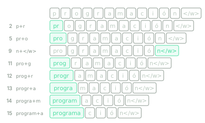
"programación" coming down the merge list. On the left, the number of the merge that fires each row and the pair it glues; in green, the piece that has just been formed. Thirteen pieces at the start, five at the end.
And the result, which is what the model ends up seeing:
>>> encode("programación", merges)
('programa', 'c', 'i', 'ó', 'n</w>')
Five pieces, and only the first means anything on its own. Behind it are the loose letters of the
ending, unmerged, because fifteen merges only stretch so far: the list ran out of budget before it
got to them. Keep training and that changes. Nine merges later, number 24 glues programació to
n</w> and the whole word becomes a single token, from five down to one.
There, in miniature, is the trade-off everything else is about. Every merge you add shortens the sequences and costs a vocabulary entry, with its two rows of numbers. Nobody writes the rule for where to stop: you pick a number of merges, and the algorithm uses it to decide which words of the language fit whole and which reach the model in pieces.
That the order rules has two consequences worth seeing together. The good one is determinism, which is the other condition a tokeniser has to meet: the same word always produces the same cut, because the list does not change and is always walked the same way. If the cut changed from one day to the next, what the model learned would stop matching what it receives. The awkward one is that the list is the tokeniser right down to its silliest details. In my code, when two pairs tie on frequency the one seen first wins, and that line is as much a part of the tokeniser as the corpus is: two implementations that break ties differently, trained on the same text, produce different vocabularies and cut differently forever.
The word the corpus did not contain
That leaves the question the word tokeniser could not answer: what to do when a word arrives that the corpus did not contain. Take "El niño programa una criptomoneda", an ordinary sentence, and cut it with a word tokeniser trained on the corpus above: three of its five words are not in the vocabulary. "criptomoneda" is the worst of the three, because it is not an oddity or a proper noun, it is a normal word that this corpus happened not to contain, and about it a word tokeniser has absolutely nothing to offer.
With the same list of fifteen merges, and beside it two words the corpus did contain:
niño           -> niñ o</w>
enseñar        -> en s e ñ a r </w>
criptomoneda   -> c r i p t o m o n e d a</w>
There is no UNK anywhere. "criptomoneda" did not appear in the corpus, none of its merges were
learned, and even so the tokeniser writes it out whole, letter by letter, because single letters are
always in the vocabulary. That is the property that let BPE take over the field: the vocabulary is
closed and finite, and yet every string has a representation.
And now the price, which in 2016 did not look serious and today is half the problem. "criptomoneda" has cost twelve tokens instead of two or three. The word has not been lost, it has been made expensive, and on top of that it reaches the model chopped into pieces that mean nothing separately. The question is no longer whether a word is in . It is how much the tokeniser charges you to write it, and that question has a different answer for every language.
Three ways of choosing the pieces
BPE is the one everybody names and it is not the only one in use. There are three algorithms in production, and the difference between them fits in one sentence: what changes is the criterion by which a piece is admitted to the vocabulary. One of the three also changes the direction it is approached from.
WordPiece: merge what is sought, not what is plentiful
WordPiece runs the same greedy loop as BPE, starting from characters and merging one pair per round, and changes only the score it picks the pair by. Where BPE keeps the highest , WordPiece divides that same count by how much or how little each piece appears on its own:
where is the number of times the piece appears in the corpus, alone or accompanied, and likewise for .
Taking logarithms, the score is , which is the pair's pointwise mutual information up to a constant that is the same for every pair and therefore does not change which one wins. And that quantity measures something else: not how many times they appear together, but how many times more than you would expect if each went its own way.
The difference shows in the trace from the previous section. The third merge glued e to n because
the pair came up thirteen times, but e and n are two of the most frequent letters in Spanish:
that they coincide a lot says nothing about them. WordPiece divides by precisely that, and prefers
pairs whose pieces, taken separately, are rarer than their union suggests. The vocabulary that comes
out has less filler and more pieces that correspond to something.
It comes from a 2012 paper on voice search in Japanese and
Korean, two languages where it is
not even clear where a word ends, and it became famous six years later for being
BERT's tokeniser. It marks continuations with ##: in
c ##ript ##omo ##ned ##a, the ## says that piece does not start a word, and removing it
reconstructs the text.
There is a second difference that almost nobody mentions. WordPiece keeps no merge list. BPE encodes by replaying its own in order; WordPiece, which no longer has one, encodes another way: at each position it takes the longest piece in the vocabulary that fits there and carries on from where it ends. Two nearly identical training algorithms that produce two different encoders.
Unigram: start at the top and prune
The third one inverts the whole direction. Instead of growing from the alphabet, it starts with an enormous vocabulary of candidates (every reasonably frequent substring of the corpus) and removes the ones that are least needed, until it comes down to the fixed size.
Deciding which are least needed forces you to measure it, and measuring it forces you to have a model. That is the underlying difference from the other two. A segmentation of a sentence has probability
that is, each piece has its own and they are assumed not to depend on one another: hence unigram. With that, the best segmentation of a sentence is the one with the highest .
Finding it is cheaper than it looks. A string of characters can be split into contiguous pieces
in ways, so enumerating them is out of the question for any real sentence, but nothing
needs enumerating. Taking logarithms, is a sum of terms that do not affect one
another, and then the best way of cutting through to position depends only on the best way of
reaching each earlier position , plus the score of the piece running from to . You walk the
sentence left to right keeping one number per position, the best accumulated score up to there, and
at the end you retrace the path backwards. That walk has a name: it is the Viterbi algorithm, the
same one used to decode hidden Markov models, and it changes the cost from exponential to
, with the length of the longest piece in the vocabulary. It is exactly the code a
few paragraphs below, where is called maxlen.
Training, for its part, now has something to optimise: the likelihood of the corpus, summing over all possible segmentations of each sentence ,
The algorithm alternates two steps. The first adjusts the , and has a chicken-and-egg difficulty: to know how much each piece is used you would need to know where each sentence is cut, and to cut the sentences you need the . It is broken with expectation-maximisation (EM), which goes back and forth between the two halves: with the from the previous round it computes how many times each piece is expected to appear, counting every possible segmentation weighted by its probability, and sets the new proportional to those expected counts. The second step computes, piece by piece, how far would fall if that piece did not exist, and throws out the ones that cost least. Round again, down to the fixed size.
It comes from a 2018 paper whose main subject is, in fact, something else. Because the model gives probabilities, there is no single good segmentation but a ranking of them, and you can sample: the same sentence goes in cut one way today and another way tomorrow, which works as data augmentation and makes the model less brittle in the face of an odd cut. Neither BPE nor WordPiece can do that, because for them only one answer exists.
The file gives it away
None of this has to be taken on faith. Any open model's tokeniser is a file you can download and open, and what is inside gives the algorithm away:
| algorithm | what the file carries | example |
|---|---|---|
| BPE | vocabulary and an ordered merge list | GPT-2: 50,257 entries, 50,000 merges |
| WordPiece | a bare vocabulary, no merges, with the ## prefix declared | BERT: 30,522 entries |
| Unigram | a vocabulary where each piece carries its | XLM-R: 250,002 scored entries |
The arithmetic in the first row adds up on its own and is worth a look: . Two hundred and fifty-six starting pieces, fifty thousand learned merges and one special end-of-text token. Where those 256 come from is exactly the subject of the next section.
The scores in the third row are literal: in XLM-R's vocabulary, ▁de is worth , ción is
worth and ▁niño is worth , where ▁ marks that the piece starts a word. With those
numbers and fifteen lines of Python you can reproduce the entire tokeniser.
def segment(text, pieces, maxlen=16):
    # Viterbi: of all the ways of splitting the text into vocabulary pieces,
    # the one maximising the sum of log p(x). Cost O(n * maxlen), not exponential.
    s = "▁" + text.replace(" ", "▁")
    n = len(s)
    best = [-math.inf] * (n + 1)      # best log-probability up to position j
    back = [0] * (n + 1)              # where that optimum came from, to rebuild it
    best[0] = 0.0
    for j in range(1, n + 1):
        for i in range(max(0, j - maxlen), j):
            p = pieces.get(s[i:j])    # None if that substring is not a piece
            if p is not None and best[i] + p > best[j]:
                best[j], back[j] = best[i] + p, i
    out, j = [], n
    while j > 0:
        out.append(s[back[j]:j])
        j = back[j]
    return out[::-1]
Load XLM-R's published vocabulary into pieces and this function returns exactly what the official
tokeniser returns, token for token. It does not resemble the algorithm: it is the algorithm.
The three on the same words
With the three real tokenisers in front of you, cutting the same six Spanish words:
| word | BPE (GPT-4o) | WordPiece (mBERT) | Unigram (XLM-R) |
|---|---|---|---|
| niño | ni ño | niño | ▁niño |
| jardín | j ard ín | jardín | ▁jardí n |
| enseñar | ense ñar | ens ##eña ##r | ▁enseñar |
| programación | program ación | programación | ▁programación |
| dámelo | d ám elo | dá ##mel ##o | ▁dám elo |
| criptomoneda | cript omon eda | c ##ript ##omo ##ned ##a | ▁cripto mone da |
The comparison is not clean and it is worth saying so: the three vocabularies are of very different sizes (200,019, 119,547 and 250,002) and were trained on different corpora, so what you see is not the algorithm alone. Even so, two things read off without effort.
No two of them agree on any of the words they break into pieces. And none of the three finds the
segmentation a speaker would give for "dámelo", which is "dá me lo", the imperative with its two
clitics: out come d ám elo, dá ##mel ##o and ▁dám elo. Three algorithms, three cuts, and all
three the same distance from morphology. Pieces look like morphemes when the morphemes are frequent,
and like nothing recognisable when they are not; the previous section already flagged it with a
single tokeniser, and here you can see it was not that one's fault.
SentencePiece is not a fourth algorithm
It is the most repeated confusion in the subject, and it comes from the name appearing on the spec sheet of half a dozen models. SentencePiece is an implementation: a library that trains and applies BPE or Unigram, not a third way of choosing pieces. Saying a model "uses SentencePiece" tells you as little as saying a program "uses gcc".
What it did contribute, and it is what made it take over, is of a different order. Earlier tokenisers
assumed the text arrived already split into words by a separate program, with its per-language rules,
the same ones from the first section. SentencePiece skips that step: it treats the sentence as a
stream of characters, spaces included, and turns the space into one more symbol, the ▁ in the table
above. With that there are no per-language rules to maintain, Japanese and Spanish come in through
the same door, and reconstruction is exact again with no conventions to remember: glue the pieces,
swap ▁ back for a space and you have the text you started with.
Even so, the three algorithms share an assumption we have not touched yet. All three build their pieces out of characters, and which characters exist is decided by looking at the corpus. If a text turns up tomorrow with one that corpus did not have (an emoji, an ideogram, a letter from an alphabet nobody considered), the vocabulary comes up short again. It is the same hole as before, one floor down.
The byte floor
Unicode has on the order of 150,000 characters assigned, spread across more than 150 writing systems, and more are added every year. No corpus contains them all. So the alphabet any of the three algorithms starts from, however large the corpus, is always an incomplete list, and the problem from the first section reappears one floor down: along comes an ideogram, an emoji invented last year or a letter from an alphabet nobody looked at, and the tokeniser has nothing to write it with.
The solution that won out, and that arrived with GPT-2 in 2019, is uncomfortably simple: stop building the pieces out of characters and build them out of bytes. Any text, in any script, is stored on disk as a sequence of UTF-8 bytes, and a byte can take only 256 values. If the starting alphabet is those 256, there is no text that cannot be written with the vocabulary. None. Ever.
That is where the arithmetic from the previous section fits: . The 256
bytes, the 50,000 merges learned on top of them and one end-of-text token. GPT-2's vocabulary has
no unknown token, and not by oversight: it does not need one, because nothing can be left out. The
UNK that had forced people to invent patch-up dictionaries disappears from the problem by
construction.
What going down to the byte costs
A floor made of bytes has an odd consequence: a token can be a piece of a character. Not an incomplete letter in some figurative sense, but a sequence of bytes that on its own is nothing.
'🙂'   its UTF-8 bytes are  b'\xf0\x9f\x99\x82'
  gpt2          2 tokens:  [b'\xf0\x9f', b'\x99\x82']
  cl100k_base   2 tokens:  [b'\xf0\x9f', b'\x99\x82']
  o200k_base    1 token:   [b'\xf0\x9f\x99\x82']

'漢字'  its UTF-8 bytes are  b'\xe6\xbc\xa2\xe5\xad\x97'
  gpt2          5 tokens:  [b'\xe6', b'\xbc', b'\xa2', b'\xe5\xad', b'\x97']
  cl100k_base   3 tokens:  [b'\xe6\xbc', b'\xa2', b'\xe5\xad\x97']
  o200k_base    2 tokens:  [b'\xe6\xbc\xa2', b'\xe5\xad\x97']
With GPT-2, the smiley costs two tokens and neither of them is a character: b'\xf0\x9f' is the first
half of an emoji, and on its own it cannot even be printed. The two ideograms cost five tokens, three
of them loose bytes. The model does not see two characters, it sees five pieces whose relationship to
what was written exists only if it learns to reconstruct it.
That is the currency the guarantee is paid in. Nothing falls outside the vocabulary, but whatever is
far from the training corpus comes in chopped into meaningless fragments. Compare it with ñ, which
in all three tokenisers is a whole token despite taking two bytes: Spanish is represented well enough
in the corpus for that merge to have been learned. The difference between a cheap character and an
expensive one is not Unicode, it is how much it turned up in the corpus.
The regex almost nobody looks at
Before BPE touches the text there is a step almost nobody talks about, and it decides more than it looks. The text is first split with a regular expression, and merges can never cross those cuts. The regex, therefore, speeds nothing up: it delimits what the algorithm is allowed to learn.
The part governing numbers changed between generations, and you can see it at a glance:
| tokeniser | digits in the regex | 1234567 | 2026 |
|---|---|---|---|
| gpt2 | ' ?\p{N}++', runs of any length | 123 45 67 | 20 26 |
| cl100k, o200k | '\p{N}{1,3}', groups of three at most | 123 456 7 | 202 6 |
In GPT-2 the regex handed over 1234567 whole and BPE merged inside it according to what it had
seen, so the cuts landed wherever they landed. From cl100k on, the cut comes first and is fixed:
groups of three, left to right. Look at what that does to the year I am writing this in. 2026 is
not split into 20 and 26, nor left whole: out come 202 and 6. The same digit ends up in a
different token depending on the length of the number around it, and that decision, taken in a
regular expression, is where half of language models' arithmetic problems come from.
Two roads to the same floor
Not everyone went down to the byte through GPT-2's door. SentencePiece, which trains on characters,
added an option called byte_fallback: the vocabulary stays a vocabulary of characters, and only
when one turns up that is not there does it fall back on writing it out with its bytes. The guarantee
is the same, the route is not.
Llama's two tokenisers show both routes, one per version. Llama 2's, with 32,000 pieces, declares
byte_fallback: true: it is a character BPE with a safety net. Llama 3's, with 128,256, declares it
false, and not because they removed the net, but because it is no longer needed: they switched to
byte BPE, where the floor is the alphabet itself. In two versions of the same family you can see the
whole migration.
The vocabulary race
With the floor settled, the question from above remains: how many pieces. And here the numbers moved a great deal in a few years, from Llama 2's 32,000 to GPT-4o's 200,019.
What going up buys is sequence length. What it costs is parameters: the model stores the embedding matrix and the output one, numbers in total, and the final layer does on the order of operations for every token it generates. With and , those two matrices come to about 1,050 million parameters, which in an eight-billion model is more than an eighth of the total spent getting in and out of the vocabulary. Raising divides the number of steps and multiplies the cost of each one, so there is an optimum and it depends on the size of the model; there is recent work devoted to locating exactly that.
While we are looking at numbers, the interesting question is what that size buys for Spanish. Here are seven real tokenisers on the same text, 400,000 characters of Spanish literature, 72,786 words:
| tokeniser | algorithm | tokens per word | |
|---|---|---|---|
| Llama 2 (2023) | BPE + byte_fallback | 32,000 | 1.750 |
| GPT-2 (2019) | byte BPE | 50,257 | 2.029 |
| GPT-3.5 and GPT-4 (2022) | byte BPE | 100,277 | 1.653 |
| multilingual BERT (2018) | WordPiece | 119,547 | 1.542 |
| Llama 3 (2024) | byte BPE | 128,256 | 1.650 |
| GPT-4o (2024) | byte BPE | 200,019 | 1.460 |
| XLM-R (2019) | Unigram | 250,002 | 1.519 |
Within one family the trend is clean: OpenAI's three tokenisers bring Spanish down from 2.03 to 1.65 and then 1.46 tokens per word as they double the vocabulary, with clear diminishing returns (the first doubling takes 18%, the second 12%).
Across families, the table says something different and more useful. Size does not rule. Llama 2, with 32,000 pieces, cuts Spanish better than GPT-2 with 50,257. A multilingual BERT from 2018 cuts it better than a Llama 3 from 2024, at almost the same vocabulary size. And XLM-R, with 250,002 pieces, the largest vocabulary in the table, loses to GPT-4o, which has fifty thousand fewer.
What decides it is not how many pieces there are, but how many of them were spent on your language. XLM-R spreads a quarter of a million pieces across a hundred languages; GPT-4o concentrates two hundred thousand on rather fewer. A vocabulary is a budget, and dividing it up is a product decision nobody consults you about and that you end up paying for by the token.
What the choice costs you
Everything above is machinery. This section is the bill, and the point of it is that none of what follows is a mystery: each one can be traced back to a concrete decision you have watched being taken in the earlier sections.
The tax on writing in Spanish
Take the Quijote in Spanish and Ormsby's English translation, both on Project Gutenberg, and run OpenAI's three tokenisers over each. The Spanish original takes 2,105,831 characters; the English translation, 2,292,068. The Spanish text is shorter.
| tokeniser | tokens in Spanish | tokens in English | Spanish / English | characters per token, es / en |
|---|---|---|---|---|
| gpt2 (2019) | 778,102 | 565,416 | 1.38 | 2.71 / 4.05 |
| cl100k (2022) | 632,915 | 541,068 | 1.17 | 3.33 / 4.24 |
| o200k (2024) | 558,227 | 536,900 | 1.04 | 3.77 / 4.27 |
With GPT-2, the shorter book costs 38% more. The right-hand column says why: the tokeniser gets 4.05 characters out of every token in English and 2.71 in Spanish, so the same reading effort yields half as much. And that difference is not merely cosmetic, because tokens are the unit everything else is counted in: what fits in the context window, how long a reply takes and what the API bill comes to. Writing in Spanish was, literally, more expensive.
The last row is the good news this article opened with: with GPT-4o's tokeniser the ratio drops to 1.04, near parity. Not because Spanish changed, but because doubling the vocabulary left room to put whole Spanish words inside it. And it is worth not generalising from here to every language: Spanish shares an alphabet with English and turns up in training corpora by the bucketload. For languages that also change script, the difference is still a matter of several factors, and the byte-floor section explains why: when one character costs three tokens of loose bytes, no vocabulary fixes that without devoting space to it.
Why it cannot count the r's in a word
It is the example that circulates everywhere, and it is almost always explained wrongly. The question is how many r's there are in "strawberry", and the model gets it wrong. The cause is not that it cannot count:
strawberry    ->  str · aw · berry
ferrocarril   ->  fer · roc · arr · il
The model never sees the word. It sees three pieces, and not one of the three is a letter. To answer
it would have to know by heart how each piece is spelled, because the information it needs was
destroyed before it existed, at the moment of the cut. In Spanish the same thing happens and worse:
"ferrocarril" has four r's spread across four pieces, and one of them, arr, carries two inside it.
Counting over that is counting over something that is not there.
It is the condition from the first section seen from the other side. The tokeniser can preserve the whole text and still destroy the structure of the text, because preserving and making accessible are not the same thing.
Arithmetic, cut in the wrong places
The regex from the previous section splits digits into groups of three from left to right. Look at it on numbers that resemble each other closely:
1000    ->  100 · 0
10000   ->  100 · 00
100000  ->  100 · 000
1999    ->  199 · 9
19999   ->  199 · 99
The first digit of 1000 is in the same token as the second and third, and the last one goes alone.
In 10000, that same leading 100 is now followed by 00. The tokens do not correspond to units,
tens and hundreds, and they fail to correspond differently depending on the length of the number. A
model doing addition has to do it over pieces whose position within the number changes from one case
to the next. That arithmetic on long numbers is fragile stops being a mystery the moment you see the
cuts: it is not adding digits, it is predicting fragments.
The space at the end of the prompt
This one bites anyone programming against an API, and it is completely invisible:
'El niño juega en el'    ->  El · ni · ño · jue · ga · en · el
'El niño juega en el '   ->  El · ni · ño · jue · ga · en · el · ␣
One extra space at the end of the prompt adds a token that exists on its own. And here is the
problem: in all the text the model was trained on, the space goes glued to the following word
( jardín, with its leading space, is one token). A loose space at the end is a situation the model
has hardly ever seen, so instead of continuing with jardín it has to continue with something that
starts without a space, which is a completely different distribution of probability. One extra
keystroke and quality drops. Some libraries fix it internally with what is called token healing:
they remove the last token of the prompt and merge it again with whatever the model generates. Almost
none does it by default.
Indentation, and why code got cheaper
The same mechanism explains a change that people did notice at the time. One indented line of Python, under GPT-2 and under cl100k:
'    return x'      gpt2   5 tokens:  ␣ · ␣ · ␣ · ' return' · ' x'
                    cl100k 3 tokens:  '   ' · ' return' · ' x'
'        return x'  gpt2   9 tokens
                    cl100k 3 tokens
GPT-2 spent one token per space, so a function with eight levels of nothing ate the context window in indentation. cl100k put pieces of several consecutive spaces into the vocabulary and the same code came to cost half as much or less. Nobody changed the model: they changed what was on the list.
The ghost tokens
The strangest of the lot, and the one that best shows the tokeniser is a separate component. GPT-2's
vocabulary contains entries like SolidGoldMagikarp, petertodd, RandomRedditor and
externalToEVAOnly, each a single token. They are Reddit usernames and code fragments that
appeared so relentlessly in the material the tokeniser was trained on that they earned their merge.
The catch is that this material is not the same as the material the model was trained on. When those
texts were filtered out of the training corpus, their tokens stayed in the vocabulary with an
embedding row initialised at random and never adjusted. Asking GPT-2 to repeat one of them
produced absurd or evasive replies,
because it was reading a vector that meant nothing. Most of them disappeared from later vocabularies,
though not all: davidjl is still a single token in GPT-4's.
Not one of these six things is a programming error. All of them are the consequence of a reasonable decision: compress the corpus you had, cut numbers in a fixed way, put spaces inside the following word, use the text available to train the tokeniser. What they have in common is that none of them was taken with any thought for what you were going to do with the model.
What comes after the tokeniser
After seven sections of problems caused by choosing a unit, the question is ripe for the picking: why not take the tokeniser out of the way and let the model read bytes.
It has been tried, and it works. ByT5 is a 2021 model that reads raw bytes and holds its own against its tokenised version, besides being far more robust to typos, which is exactly what you would expect from something that sees the letters. CANINE, from the same year, does something similar by compressing the sequence internally. Both run into the wall from the third section: without long units the sequence is multiplied by six and the cost by thirty, and no amount of elegance pays for that.
What has changed in recent years is the shape of the question. Instead of choosing between a large unit and a small one, the idea is not to fix the unit at all: let the model read bytes and decide on the fly where to group them. MEGABYTE did it with fixed-size patches. The Byte Latent Transformer, from late 2024, does it with variable-size patches, and its criterion is the best idea in the whole business: a small model estimates the entropy of the next byte, and a new patch is opened where that entropy spikes,
Read it slowly, because it inverts the entire premise of the article. BPE spends pieces where the corpus repeated things, years ago and once and for all. This spends compute where the text in front of you is hard to predict, now. The end of "programación" is predictable and does not deserve a cut; the proper noun you have never seen deserves several. A tokeniser that adapts to the text instead of to a frozen corpus.
At the other extreme there are people pushing the opposite way, and doing well out of it: SuperBPE keeps the vocabulary fixed but lets pieces cross spaces, so that whole expressions become one token. And H-Net learns the chunking end to end, inside the network, with no separate module at all.
As of today none of this is the norm. The models you use when you open an API have a byte BPE inside them with a vocabulary of between one and two hundred thousand pieces, trained once and frozen. What would have to happen for that to change is measurable: the overhead of reading longer sequences would have to fall below what the fixed vocabulary costs today, counting into that cost the billion parameters of the two matrices, the per-language tax and the list of defects in the previous section. It is closer than it was three years ago. I am writing this in 2026, and it is the part of the article that will age worst.
What you take away
If you take one thing away, let it be this: the tokeniser is the only part of the system that is decided before anything is learned and is never revisited. Everything else in a language model is adjusted from the data. The cut is not. It is fixed at the start, with whatever corpus existed then, and everything it discards or scrambles stays discarded and scrambled forever.
And if you take three more, let them be practical.
Measure your own text before choosing a model. The table in the byte-floor section is built from seventeenth-century literature; your text looks nothing like that. It is six lines:
import tiktoken

enc = tiktoken.get_encoding("o200k_base")     # or "cl100k_base", to compare
text = open("what_you_write.txt", encoding="utf8").read()
tokens, words = len(enc.encode(text)), len(text.split())
print(f"{tokens / words:.2f} tokens per word")
Between 1.46 and 2.03 tokens per word, which is the range this article gets for the same Spanish text, there is a 40% difference in what fits in the context, in how long it takes and in what it costs. It is worth knowing where in that range you sit before signing anything.
Treat the prompt as what it is, a sequence of tokens. Do not leave a loose space at the end. Do not expect reliable arithmetic on long numbers. Do not ask it to count letters, because it does not have them in front of it. None of those three is a flaw in the model that a better version will fix: they are consequences of the cut, and they are only fixed by changing the cut.
And if you ever train something of your own, start there. A tokeniser trained on your own domain, however small, cuts better than a general-purpose one with ten times the pieces, for the same reason a multilingual BERT from 2018 cuts Spanish better than a Llama 3 from 2024: what decides it is not how many pieces there are, but how many were spent on what you write.
Back to the beginning. "El niño juega en el jardín." It cost twelve tokens in 2019 and costs seven now, the same as in English. Nobody fixed Spanish. What changed was who got on a list.