 By Gustavo Torres
An online shop has a customers table with 200,000 rows and an orders table with 3 million. Some time ago someone created an index on the column that links them, the customer id in the orders table, precisely so that JOINs would be fast. This query adds up what the customers in Soria have bought:
SELECT count(*) AS pedidos, sum(p.importe) AS facturado
FROM clientes c
JOIN pedidos p ON p.cliente_id = c.id
WHERE c.provincia = 'Soria';
The shop is Spanish, and so is its schema: clientes are the customers, pedidos the orders,
importe the amount of an order, and provincia the customer's province, one of Spain's 52.
Soria is the least populated of them; Madrid, the most.
Postgres runs the query the way it's taught in class: it takes the 339 customers in Soria and,
for each one, looks up their orders in the index. It takes 31 milliseconds. Change 'Soria' to
'Madrid' and the plan changes completely: Postgres reads the 3 million orders from start to
finish and doesn't touch the index. It looks like an oversight, so you can force it to use the
index (how comes later). It takes 1.4 seconds, instead of 0.7.
| Looking up the index | Reading both tables in full | What Postgres picks | |
|---|---|---|---|
| Soria (339 customers) | 31 ms | 457 ms | the index |
| Madrid (28,804 customers) | 1.4 s | 0.72 s | the full tables |
The query is the same, and so is the index. What changes is how many rows come out of the filter, and with that, which way of running the JOIN is cheap.
The way a JOIN is usually taught is the one that just worked for Soria: for each row of one table, look up the rows with the same value in the other. Without an index that costs comparisons; with an index, . It isn't wrong, but it describes one of the three algorithms a database has for running a JOIN, the nested loop, and it's precisely the one Postgres ruled out for Madrid. The other two, the hash join and the merge join, don't look anything up row by row. Which one runs is decided by the optimizer, the part of the database that, before running a query, considers several possible plans, estimates what each would cost and keeps the cheapest. It estimates, it doesn't measure, and much of what follows comes from that difference.
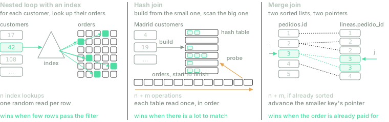
The three JOIN algorithms. The first is the one usually taught; the other two don't look anything up row by row. is the number of rows of the small input and that of the big one.
Every number in this post is measured. The shop is invented: customers are spread across provinces like the population, and 2 % of them are businesses, which buy quite a lot more than an individual (this will matter). The script that generates it is public and uses fixed seeds, so it produces exactly the same rows on any Postgres 18, and anyone can repeat the measurements. The queries run on Postgres 18.6, in Docker, on a four-core laptop with a SATA SSD, with parallelism turned off so that each plan reads in one go. Every time is the median of three runs. The timings depend a lot on where the data is, and that has its own section further down; until then, all the Postgres ones use its default memory, on a machine where the database files fit in the operating system's memory.
What SQL says, and what it doesn't
The result of clientes JOIN pedidos ON p.cliente_id = c.id is defined like this: form every
possible pair of a customer and an order, and keep the ones that meet the condition. With
200,000 customers and 3 million orders that's 600 billion pairs. That's where the
comes from: it's the definition of the result, not the way to compute it. No engine forms those
pairs, just as nobody sorts a list by comparing each element with all the others, even though
sorting can be defined that way.
SQL is declarative: the query says which rows you want, not how to find them, just as
ORDER BY doesn't say which sorting algorithm to use. Between the query and the result there's a
plan, and the plan is decided by the optimizer. For a JOIN of two tables it has to decide three
things: how to read each table (in full or through an index), which algorithm to join them with,
and which table goes on the outside. With more tables, also the order in which to join them.
You see the plan with EXPLAIN, which shows it without running the query, and with
EXPLAIN ANALYZE, which runs it and puts what actually happened next to each estimate. This is
the plan for Soria, trimmed to what matters:
Nested Loop  (rows=6600) (actual rows=5372.00 loops=1)
  ->  Seq Scan on clientes c  (rows=440) (actual rows=339.00 loops=1)
        Filter: (provincia = 'Soria'::text)
  ->  Bitmap Heap Scan on pedidos p  (rows=31) (actual rows=15.85 loops=339)
        Recheck Cond: (c.id = cliente_id)
        ->  Bitmap Index Scan on pedidos_cliente_id_idx  (rows=31) (actual rows=15.85 loops=339)
              Index Cond: (cliente_id = c.id)
It reads as a tree. Each line with -> is an operation, its children go below it and further
indented, and rows flow up from the leaves to the root. The root is the JOIN, a Nested Loop
with two children. The first, the outer one, reads the whole clientes table (a Seq Scan,
sequential scan) and keeps the customers in Soria. The second, the inner one, fetches a
customer's orders in two steps: the Bitmap Index Scan looks up in the index where they are,
and the Bitmap Heap Scan goes to read them from the table, after sorting those positions by
page so as not to read any page twice. Each node carries two row counts: rows is what the
optimizer estimated before starting, and actual rows what really came out, on average per run;
loops says how many times the node ran. The two inner nodes have loops=339: they ran once for
each customer in Soria and returned 15.85 orders on average. It's, literally, the algorithm we
started from. The optimizer expected 440 customers and 31 orders per customer. The first is
close to the real 339. The second will come back.
Nested loop: the loop you already knew
The simplest version is two loops, one inside the other:
for c in clientes:              # the outer table
    for p in pedidos:           # the inner one, in full, once per customer
        if p.cliente_id == c.id:
            emit(c, p)
For the 339 customers in Soria that's a billion comparisons, so nobody uses it between large
tables. But it has something the other two algorithms don't: it accepts any condition. The hash
join only works for equalities, and so does Postgres's merge join. A JOIN with
ON p.fecha BETWEEN c.alta AND c.alta + 30 (orders placed in a customer's first 30 days), or
with ON t.text LIKE f.pattern, can't be run with either of them, and if on top of that there's
no index that serves the condition, the nested loop is all that's left.
The second version saves reads, not comparisons. Instead of scanning the inner table once per row of the outer one, it reads the outer table in blocks that fit in memory and scans the inner one once per block: if a thousand customers fit in each block, the orders table is read a thousand times fewer. That's the block nested loop, and it was MySQL's fallback for JOINs without an index until 2019.
The third version, the nested loop with an index, is the one from the opening: replace the inner loop with an index lookup.
for c in clientes:
    for position in pedidos_cliente_id_idx.lookup(c.id):   # walk down the tree
        p = read_row(pedidos, position)                     # and fetch each order
        emit(c, p)
A Postgres index is a B-tree: the values of cliente_id, sorted and spread over 8 KB pages,
with branch pages above them that say which page to go to next. The one on
pedidos.cliente_id has three levels for 3 million values, so finding a customer's orders costs
walking down three pages. That's the , and the count is right, but it leaves out
what costs the most. The index doesn't store the orders; it stores where they are. For every
match you have to go and read the row from the table page it lives on, and the orders were
stored as they arrived, in date order: a customer's orders are scattered across the 22,059 pages
the table takes up. For Soria that's 5,372 orders, almost each one on a different page. For
Madrid, 431,921. The Bitmap Heap Scan in the Soria plan sorts each customer's positions by
page, but between one customer and the next the pages are anywhere again.
That decides when the nested loop with an index wins: when few rows come out of the outer side,
because its cost grows with them and not with the size of the inner table. Soria is the textbook
case. It also wins with a LIMIT, because it can stop as soon as it has the first rows, and when
the condition isn't an equality.
Hash join: read each table once
The plan for Madrid is a different one:
Hash Join  (rows=430095) (actual rows=431921.00 loops=1)
  Hash Cond: (p.cliente_id = c.id)
  ->  Seq Scan on pedidos p  (rows=3000000) (actual rows=3000000.00 loops=1)
  ->  Hash  (rows=28673) (actual rows=28804.00 loops=1)
        Buckets: 32768  Batches: 1  Memory Usage: 1269kB
        ->  Seq Scan on clientes c  (rows=28673) (actual rows=28804.00 loops=1)
              Filter: (provincia = 'Madrid'::text)
No node has loops greater than 1: each table is read only once. The algorithm has two phases.
In the build phase, it reads the small input, the 28,804 customers in Madrid, and puts each
id into a hash table in memory (1.2 MB, according to the plan). In the probe phase, it
scans the big input from start to finish and, for each order, computes the hash of its
cliente_id and checks whether it's in the table. Checking costs the same whether the table
holds thirty customers or thirty thousand.
table = {}
for c in clientes_madrid:                 # build, from the small input
    table.setdefault(c.id, []).append(c)
for p in pedidos:                         # probe, with the big one, start to finish
    for c in table.get(p.cliente_id, []):
        emit(c, p)
The cost is , and here's the interesting part. If you only count operations, the
nested loop should win for Madrid: 28,804 lookups of about 22 steps each ( of 3 million)
are about 620,000 comparisons, plus 431,921 rows to fetch from the table; a little over a million
operations, against the more than 3 million probes of the hash join. It loses, 1.4 s to 0.72,
because what costs is not the operations but the pages. The hash join reads the 22,059 pages
of pedidos one after the other, and reading in order is the cheapest thing there is: Postgres
asks for pages many at a time, the next one is already on its way when it's done with the
previous one, and each page is touched only once. The nested loop asks for 431,921 rows scattered
across the whole table, each on its own page, many pages more than once, and each request waits
for the previous one to finish. The optimizer counts, above all, pages, and it tells apart the
ones read in order from the ones read at random.
The hash join has two limits. It only works for equalities: a hash table can answer "is this
value here?", not "which values fall between these two?". And the table has to fit in the memory
Postgres gives each operation, work_mem, which is 4 MB by default. If it doesn't fit, it splits
both inputs into batches by the hash of the key, writes them to disk and joins them batch by
batch; the plan flags it with Batches greater than 1. That's why it matters which input is used
to build: the small one, counted after applying the filters. Postgres built with the Madrid
customers and scanned the orders, not the other way round, and the order in which the tables are
written in the query makes no difference.
Merge join: two sorted lists
If both inputs come sorted by the key, joining them is like merging two sorted lists: a pointer on each, you advance the one pointing at the smaller value, and when both match, you emit the pair.
i = j = 0
while i < len(pedidos) and j < len(lineas):
    if pedidos[i].id < lineas[j].pedido_id:
        i += 1
    elif pedidos[i].id > lineas[j].pedido_id:
        j += 1
    else:
        emit(pedidos[i], lineas[j])
        j += 1          # an order has several lines: only j moves on
It goes through each input once, , with no hash table and almost no memory. If the inputs don't come sorted they have to be sorted first, and that costs and memory, or disk. So the merge join wins when the order is already paid for: because there's an index (a B-tree keeps its keys sorted), because the table is stored in that order, or because the query has to sort anyway.
The shop has a third table, lineas_pedido, with the 7,498,570 order lines (each with a
cantidad, quantity, and a precio, price) and a primary key (pedido_id, linea). This query
recomputes each order's total from its lines, in order-id order, which is what you do to check
that the stored amount adds up:
SELECT p.id, p.importe, sum(l.cantidad * l.precio) AS total_lineas
FROM pedidos p
JOIN lineas_pedido l ON l.pedido_id = p.id
GROUP BY p.id
ORDER BY p.id;
GroupAggregate (rows=3000000) (actual rows=3000000.00 loops=1)
Group Key: p.id
-> Merge Join (rows=7498532) (actual rows=7498570.00 loops=1)
Merge Cond: (p.id = l.pedido_id)
-> Index Scan using pedidos_pkey on pedidos p (rows=3000000) (actual rows=3000000.00 loops=1)
-> Index Scan using lineas_pedido_pkey on lineas_pedido l (rows=7498532) (actual rows=7498570.00 loops=1)There's no node that sorts. Both primary keys deliver rows in order-id order, the merge join
joins them without losing that order, the GROUP BY groups rows that already arrive together
(GroupAggregate, no hash table) and the ORDER BY comes for free. It takes 6.5 s. Forced to use
a hash join, it takes 16.4 s: the 3 million orders don't fit in the 4 MB of work_mem, so the
hash table is split into 32 batches on disk, and then 3 million orders have to be grouped with
another hash table that doesn't fit either (384 MB to disk) and the result sorted (82 MB more).
And that's why the merge join never won between customers and orders: the orders aren't sorted
by customer. The index on cliente_id could deliver them in that order, but by reading the 3
million orders in jumps, from page to page. Even with the whole table in Postgres's cache, that
takes about three seconds, whether one customer passes the filter or two hundred thousand.
How it chooses
The optimizer doesn't run the three algorithms to see which one wins: it estimates them. For that it needs to know two things, how many rows each step will move and how much each operation costs.
The rows come from the statistics that ANALYZE collects from a sample of each table. For each
column it keeps the most common values with their frequencies, a histogram of the rest and the
number of distinct values. Nobody has to remember to run it: autovacuum, a maintenance process
Postgres always keeps running (its main job is cleaning up the old row versions that UPDATE and
DELETE leave behind), runs ANALYZE on its own when roughly 10 % of a table has changed.
Between one run and the next, the optimizer works with a snapshot of the table as it was, which
is why, after loading a lot of data at once, it's worth running ANALYZE by hand. The 52
provinces are all in the most-common-values list of clientes.provincia, and that's where the
estimates of 28,673 customers for Madrid and 440 for Soria come from, close to the real 28,804 and
339. The cost comes from a cost model with a few constants: reading a page in order costs 1
(seq_page_cost), reading a scattered page costs 4 (random_page_cost), processing a row costs
0.01 (cpu_tuple_cost), and a few more. For each candidate plan, the optimizer multiplies rows
and pages by those constants, adds them up, and keeps the lowest total. For the two queries from
the opening:
| Estimated cost | Nested loop | Hash join |
|---|---|---|
| Soria | 48,475 | 64,974 |
| Madrid | 144,492 | 67,444 |
The units are "what it costs to read one page in order". The cost of the hash join barely changes from Soria to Madrid, because reading all the orders dominates it. The cost of the nested loop grows with every customer, because each one brings a few scattered pages at a price of 4.
Where is the point beyond which it pays to switch algorithms? To see it I repeated the query
varying how many customers pass the filter, from one to all 200,000 (with a random column, to be
able to pick the exact number), and measured both algorithms forced with
SET enable_hashjoin = off and SET enable_nestloop = off, which don't forbid an algorithm but
make it so expensive that the optimizer avoids it. I did it in three situations, because "reading
a scattered page" doesn't cost the same in all of them:
- In Postgres's cache. The whole database fits in the memory Postgres reserves for itself
(
shared_buffers), and it's already loaded. Reading a page is reading 8 KB of memory. - In the OS cache. Postgres with its default memory, which reserves 128 MB. The orders table, at 172 MB, doesn't fit, but its files are in the operating system's memory, and each page missing from Postgres's cache costs a system call. That's the situation of the opening timings, and that of many servers.
- On the SSD. The first run, with both caches empty and in a container limited to 160 MB so that the table fits in neither. Each scattered page is a request to the SSD.
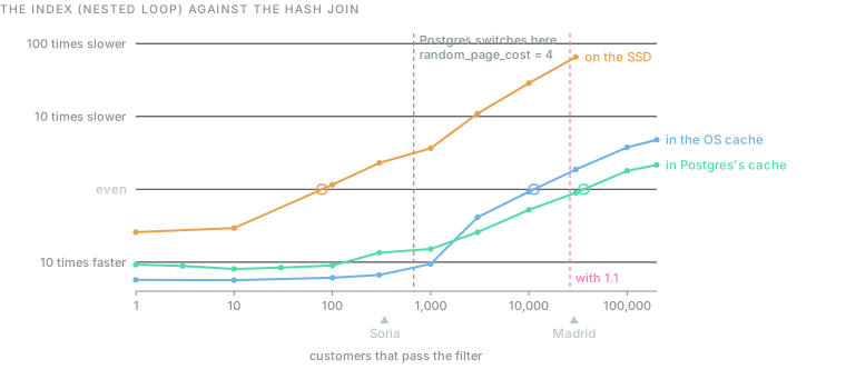
How many times slower, or faster, the nested loop with an index is than the hash join,
depending on how many customers pass the filter. Each situation crosses "even" at a different
point (the circle): about 80 customers on the SSD, 11,000 in the OS cache and 36,000 in
Postgres's cache. The grey line marks where Postgres switches algorithm with its default
settings, the same in all three cases; the pink one, where it would with
random_page_cost = 1.1. On the SSD I didn't measure the nested loop above 30,000 customers:
each run would have taken several minutes.
On the SSD, the nested loop only wins up to about 80 customers. With Soria's 339 it already takes 1.4 s against the hash join's 0.8, and with Madrid's 28,804, 61 seconds against one. In the OS cache, the crossover is around 11,000 customers, and in Postgres's cache, around 36,000: with the whole table in memory, Madrid is almost a tie (554 ms with the index, 592 without it). The real switch point moves by more than two orders of magnitude depending on where the pages are. Postgres's doesn't move: with the default values, it drops the index from 673 customers on, in all three cases.
That 673 isn't an oversight; it's placed in between on purpose. The
Postgres documentation explains
that reading a scattered page from storage normally costs much more than four reads in order, and
that 4 is lower because it assumes most scattered reads, like an index's, will find the page in
cache. It's a bet about your hardware and about how much of your data is in memory, and the
optimizer has no way of knowing, when it plans, in which of the three situations the query will
run. That's why random_page_cost can be changed, for the whole database or for a tablespace.
With 1.1, a value often recommended when the data fits in memory, Postgres drops the index from
26,161 customers on: close to the real crossover in Postgres's cache, and where on the SSD the
index is already almost sixty times slower. To get it right on this laptop's SSD it would have to
go up to about 27. No constant is right in all three cases; the sensible thing is to set it for
where your data usually lives.
With more than two tables there's one more decision, which usually weighs more than the choice
of algorithm: the order in which to join them. Counting only the plans in which each JOIN adds a
new table, tables allow orders: 120 with five tables, more than three million with ten.
The optimizer of System R, the IBM prototype SQL came out of, solved this in 1979 with
dynamic programming:
it computes the best plan for each pair of tables, then for each trio building on the best
pairs, and so on until it has them all. It also keeps the best plan for each interesting
order, a more expensive one that delivers rows sorted because a later step will take advantage
of it, like the merge join above. Postgres does the same up to eleven tables; from twelve on
(geqo_threshold) it switches to a genetic algorithm that doesn't guarantee the best order. And
there's a more practical limit: in a query with more than eight tables joined with explicit JOINs
(join_collapse_limit), Postgres stops searching among all the orders and partly keeps the one
that's written.
When it gets it wrong
The algorithms don't fail; the estimates do. In 2015, a team from the Technical University
of Munich and CWI in Amsterdam measured the optimizers of five databases
with real queries of many JOINs. They all made estimation errors of a thousand times or more,
and the errors grew exponentially with each JOIN. The Postgres queries that didn't finish almost
always had the same thing in common: a very low estimate that led it to choose a nested loop
(without an index, in their case) where there turned out to be many more rows. The shop has a
similar case. This query adds up what the businesses in Madrid have bought, line by line; tipo
is the customer type, 'empresa' for a business and 'particular' for an individual:
SELECT count(*), sum(l.cantidad * l.precio)
FROM clientes c
JOIN pedidos p       ON p.cliente_id = c.id
JOIN lineas_pedido l ON l.pedido_id  = p.id
WHERE c.tipo = 'empresa' AND c.provincia = 'Madrid';
Nested Loop (rows=22646) (actual rows=233051.00 loops=1)
-> Nested Loop (rows=9060) (actual rows=93417.00 loops=1)
-> Seq Scan on clientes c (rows=604) (actual rows=575.00 loops=1)
Filter: ((tipo = 'empresa'::text) AND (provincia = 'Madrid'::text))
-> Bitmap Heap Scan on pedidos p (rows=31) (actual rows=162.46 loops=575)
Recheck Cond: (c.id = cliente_id)
-> Bitmap Index Scan on pedidos_cliente_id_idx (rows=31) (actual rows=162.46 loops=575)
-> Index Scan using lineas_pedido_pkey on lineas_pedido l (rows=4) (actual rows=2.49 loops=93417)
Index Cond: (pedido_id = p.id)A plan like this is read from the leaves up, comparing rows with actual rows at each node
(multiplied by loops when it's greater than 1), until you find the first one where they don't
match. The businesses in Madrid: 604 estimated, 575 real, fine. The orders of each one: 31
estimated, 162 real. That's where the error is born, and it travels up from there: the optimizer
expected 9,060 orders and 93,417 come out, so the lookup in the lineas_pedido index, planned
for some nine thousand times, runs 93,417 times, each one in a different spot of a 373 MB table.
With nine thousand orders the plan was reasonable. With 93,417, what it costs depends on where
the pages are. Against the same query without nested loops (with SET enable_nestloop = off,
just to check):
| Plan chosen | No nested loops | |
|---|---|---|
| In Postgres's cache | 0.63 s | 1.4 s |
| In the OS cache | 2.3 s | 1.8 s |
| On the SSD | 58 s | 2.7 s |
With everything in memory, a scattered read is so cheap that the wrong plan is even the fastest. In the OS cache it loses by a little, nothing to raise an eyebrow. On the SSD it's twenty times slower. That's the trap in these errors: the plan that does fine in development, with test data that fits in memory, is the one that one day turns slow in production without anyone having touched the query.
The 31 has two causes. Postgres estimates the rows of a JOIN with the statistics of each column
separately: pedidos has 3 million rows and, according to its sample, 95,851 distinct values of
cliente_id (there are really 200,000), so it computes 3,000,000 / 95,851 ≈ 31 orders per
customer. The first cause is that distinct count, which comes out wrong from a sample of 30,000
rows. The second, the one that matters, is that the average applies to any customer, whatever the
filter: an individual has 12 orders and a business 162. Postgres has no way of knowing that the
tipo column in clientes says something about how many rows each customer has in pedidos,
because they are two columns in two different tables. The Munich study calls this a
join-crossing correlation, and found them everywhere in the real data it used. Fixing the
count wouldn't help: with the correct 200,000 distinct customers, the estimate would drop to 15
orders per customer, even further from 162.
What you can do:
- Look before you touch.
EXPLAIN ANALYZE, and look, from the leaves up, for the first node whererowsandactual rowsdrift apart by an order of magnitude. The wrong algorithm is almost never the cause; it's the consequence of an estimate that went wrong earlier. - If the correlation is between columns of the same table, like province and postcode,
CREATE STATISTICSfixes it: by default, the optimizer assumes conditions are independent and multiplies their probabilities, and extended statistics give it those of the columns together. - If it's between tables, no statistic fixes it. What's left is bringing the column to the
table where the skew is (if
pedidosstored the customer type, the filter would be estimated with the statistics ofpedidos), splitting the query and storing the intermediate result in a temporary table with its ownANALYZE, or forcing the algorithm for that query only, withSET LOCAL enable_nestloop = offinside a transaction. None of them is elegant.
MySQL and Oracle
With the same data loaded into MySQL 9.4, with 1 GB of cache so it all fits, the three
customers-and-orders queries (Soria, Madrid and all customers) run the same way: a nested loop
with an index lookup. MySQL only knew the nested loop, with an index or by blocks, until 8.0.18,
in 2019, when the hash join arrived;
in 8.0.20 it replaced the block nested loop altogether. But its optimizer uses it when there's no
index that serves the JOIN condition, and here there is. For Soria and Madrid it gets it right,
with the data in memory: 117 ms and 1.42 s with the index, against 1.06 s and 1.63 s with a hash
join. With all 200,000 customers it gets it wrong: 9.7 s with the index, against 2.3 s with a hash
join that has to be forced by telling it to ignore both indexes (IGNORE INDEX).
Two more details. Without histograms, which MySQL doesn't collect on its own, it assumed 10 % of
the customers were in Soria, and the same 10 % for Madrid; with
ANALYZE TABLE clientes UPDATE HISTOGRAM ON provincia it estimates 286 and 24,830, and the plan
doesn't change, because the decision didn't depend on that number. And MySQL has no merge join:
it runs the order-totals query with a loop over the primary key. MySQL has a new optimizer, the
hypergraph one, that does compare algorithms by their cost, but 9.4 refuses to turn it on outside
debug builds. In MySQL, then, the model from the opening is literally what runs: if there's an
index, it's looked up. A report that crosses whole tables can go faster without the index, and you
have to tell it so.
Oracle, which I haven't measured, has all three algorithms, with hints to ask for each one
(USE_NL, USE_HASH, USE_MERGE), and its merge join accepts inequalities. The interesting part
is what it added in version 12c, in 2013: adaptive plans.
When it hesitates between a nested loop and a hash join, it prepares both. During the first
execution, a statistics collector counts the rows arriving from the outer side; if they go past
the number at which both plans would cost the same, it switches to the hash join, and if not, it
stays with the loop. The resulting plan stays fixed for later executions. It's the direct answer
to the problem in the previous section: deciding with the rows that actually arrive, not the
estimated ones. SQL Server has an equivalent operator since 2017; Postgres, in version 18, doesn't.
In a column store
Postgres and MySQL store rows: each page holds complete rows, with all their columns. A
column store, like DuckDB, ClickHouse, Snowflake, BigQuery or Redshift, stores each column
separately, compressed and in blocks. In DuckDB, each table is split into groups of 122,880 rows,
and for each column of each group it keeps the minimum and the maximum. A query that uses two
columns of pedidos reads those two, and nothing else.
I loaded the same data into DuckDB 1.5.6, which runs inside the program itself, with everything
in memory and a single thread to compare it with Postgres, and I created the same index on
pedidos.cliente_id. The three customers-and-orders queries come out as hash joins, none uses
the index, and they take 30 ms (Soria), 41 ms (Madrid) and 42 ms (all customers). DuckDB's
documentation says it bluntly: an index doesn't change how long a JOIN takes;
it exists for key constraints and for very selective lookups. The advantage of the nested loop
with an index was not reading the whole table, and reading two numeric columns of 3 million rows,
in memory, costs a few milliseconds.
Don't read it as "DuckDB is fifty times better than Postgres": they are tools for different jobs. Postgres stores rows to be able to read, change and lock one specific order, which is what a shop does every second; DuckDB stores columns to sweep through millions of rows of a few columns, which is what a report does. And part of the difference is the format: DuckDB adds up the amounts as integers, and Postgres as arbitrary-precision decimal numbers.
What does change in a column store is where the time of a JOIN goes, and that brings two ideas worth knowing.
The first is vectorized execution. Each operator processes vectors of 2,048 values instead of one row at a time, so the hash join probes 2,048 keys in a row in a short loop the processor runs very fast. The idea comes from MonetDB/X100, in 2005. With the data in memory, the bottleneck of a JOIN stops being the disk and becomes the processor's cache: a hash table that fits in it is probed much faster than one that forces a trip to main memory on every lookup.
The second is the dynamic filter: the JOIN hands a filter to the scan of the big table. When
DuckDB finishes building the hash table, it knows the minimum and maximum of its keys and,
sometimes, it also builds a Bloom filter, a compact structure that answers, for each value,
"definitely not here" or "maybe here". With that it filters the table it's about to scan before
reading it. With each group's minimum and maximum, it can skip whole groups without opening them.
This query adds up the lines of the September orders (fecha is the order date):
SELECT count(*), sum(l.cantidad * l.precio)
FROM pedidos p
JOIN lineas_pedido l ON l.pedido_id = p.id
WHERE p.fecha >= DATE '2026-09-01';
The 82,116 September orders have ids between 2,917,885 and 3,000,000, and that's what the plan
hands to the scan of lineas_pedido:
Dynamic Filters:
  optional: pedido_id>=2917885 AND optional: pedido_id<=3000000
AND optional: pedido_id IN BF(BF is the Bloom filter.) The lines are stored in order-id order, so of the table's 65 groups
only 3 overlap that range: DuckDB reads 249,458 lines out of 7,498,570, and takes 50 ms. With
that optimization turned off it reads all 7,498,570 and takes 250 ms. In the Soria query the same
thing happens, and it's no use: the customers in Soria have ids between 116 and 197,499, and the
orders, stored in date order, have customers from the whole range in every group.
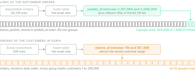
The same mechanism, with and without effect. The filter only saves reads if the big table is stored in an order that resembles that of the JOIN key: it's the column-store equivalent of choosing the right index.
DuckDB doesn't have a merge join for equalities either: it runs the order-totals query with a
hash join, a hash aggregation and a sort at the end. It keeps sort-based algorithms for JOINs on
inequalities, like ON a.fecha BETWEEN b.inicio AND b.fin, which a hash table can't handle. And
in column stores that spread the data across several machines there's one more decision, which
doesn't fit here: send the small table in full to every machine, or redistribute both by the
JOIN key.
What to take away
If you take away one thing, let it be this: the JOIN you write says which rows you want, not how to find them. "For each row, look it up in the other table" is the nested loop, one of three algorithms, and it only wins when few rows come out of one side. When there's a lot to match, reading each table once (hash join) or walking two lists that already come sorted (merge join) costs less, even though it counts more operations, because what's expensive is reading pages, and reading them scattered.
And if you take away three more, let them be practical.
An index on the JOIN column helps the nested loop, and only when few rows come out of the other side. If Postgres's optimizer ignores it in a report that crosses whole tables, it's probably right. MySQL is the opposite: it will use it even when it shouldn't.
Before changing anything, EXPLAIN ANALYZE. Look from the leaves up for the first node where
the estimated and the actual rows drift apart by an order of magnitude: that's where the problem
is, and the algorithm chosen afterwards is only its consequence. And test with production-sized
data, because in memory a wrong plan can look good.
random_page_cost is a statement about your hardware. With the default value, Postgres drops
the index from 673 customers on, whether in Postgres's cache, in the OS cache or on the SSD, when
the real point ranges from about 80 to about 36,000 depending on where the pages are. If your
database fits in memory, lowering it brings the optimizer closer to reality; if it's much larger
than memory, leave it as it is.
In a column store, what you optimize isn't indexes but how much data reaches the JOIN: filter early, and store tables sorted by the column they're filtered or joined on, so that each group's minimum and maximum are good for something.
Soria and Madrid write the same query. What changes is how many rows come out of the filter, and with that, which algorithm is cheap. The optimizer knows, or estimates; your job is to check that it estimates well.